Category Archives: Blog

So you want to distribute your music on streaming platforms?

The keywords in this question are distribute and streaming. Digital distribution is the delivery of your music to digital service providers like Spotify, Apple Music, Amazon Music, TIDAL, Napster, Google Play, Deezer, among many other streaming platforms.

Digital distribution companies (CD Baby, DistroKid, RouteNote, Mondotunes, ReverbNation, Landr, Awal, Fresh Tunes, Tunecore, Chorus Music, Symphonic, etc.) help get your music onto these digital service platforms. Without a digital distributor, the doors to these outlets are pretty much closed. That said, distribution companies do NOT own your music. They may take revenue from royalties, but you retain your rights. Distribution companies are also NOT stand-alone stores (i.e. BandCamp) although some offer this service (e.g., CD Baby).

This document is a walk-through going over the steps to digital distribution, from start to release. Over the course of the walk-through, we will create a track and then release that same track on a digital distribution service (all free). The goals of the walk-through are to:

  1. Understand the basics of digital distribution
  2. Take some of the fear out of releasing your music online
  3. Prepare for future self-release work

The walk-through should take about an hour, depending on your familiarity with audio software and a relaxed mind when it comes to generating names/titles.

The various components of releasing music in this walk-through consist of

  1. Create a track for release (we will create a pink noise track)
  2. Generate all materials associated with the release 
  3. Register with a digital distribution service (free)
  4. Distribute your work with the digital distribution service
  5. Following any additional steps you can take (PRO registration, SoundExchange, claim artist profile, digital store setup)

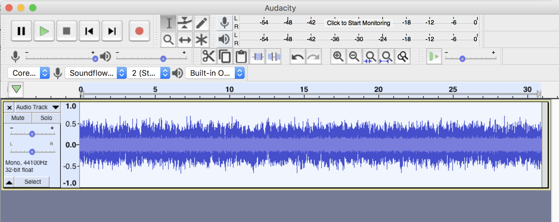
Since the hardest part of the release process is the music creation (right?), let’s just get over this hurdle by creating a noise track right now in the next five minutes. Don’t worry, we will create a pink noise track (for relaxation and sleep) to help us skirt around personal aesthetics, notions of perfectionism, genre, and all things that take time and intentional decision-making. If you have a music track already, just skip this next section.

1. CREATE A PINK NOISE TRACK FOR RELEASE

If you have a track for the release that you want to use INSTEAD of pink noise track(s), please skip this step. If not, read on. Open up Audacity (link) or any free software that can “generate” noise. Audacity is free and contains a noise generator.

Figure 1. Generate Noise menu in Audacity audio software

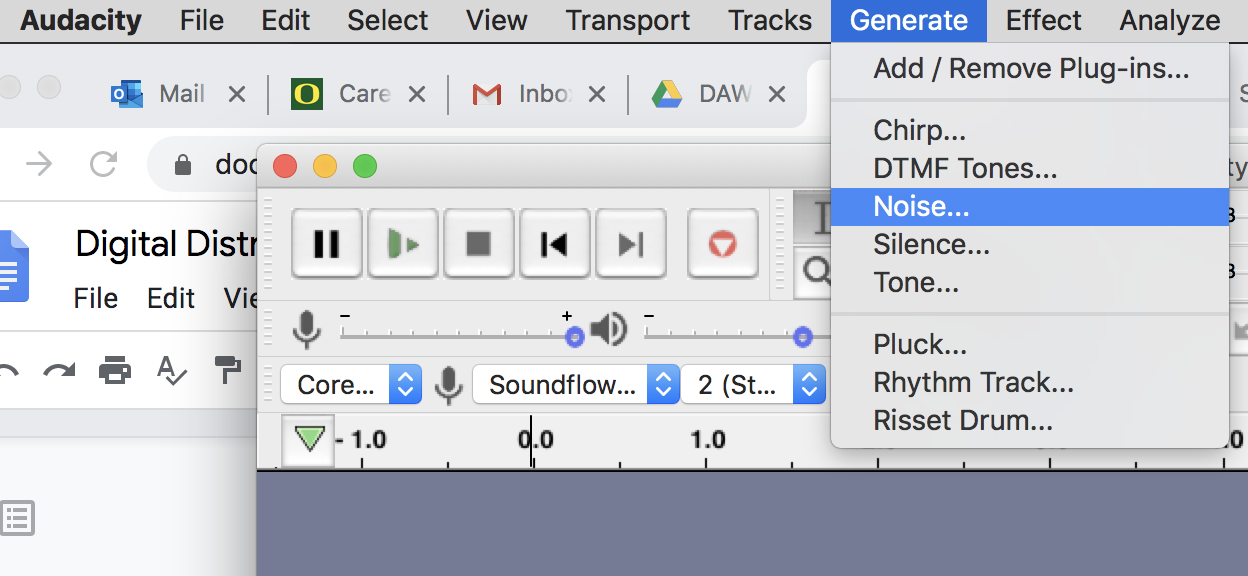
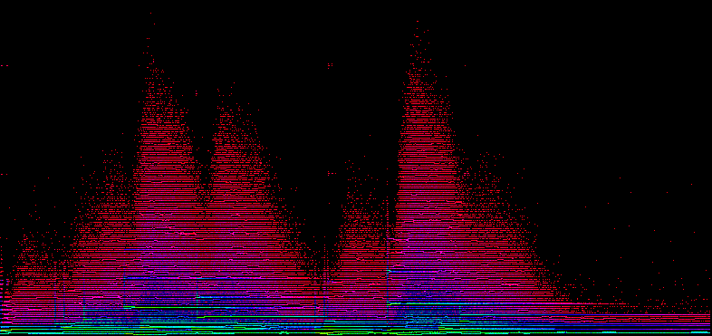
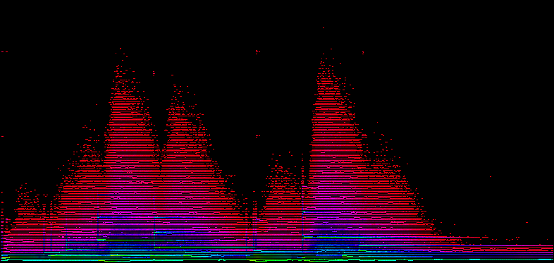
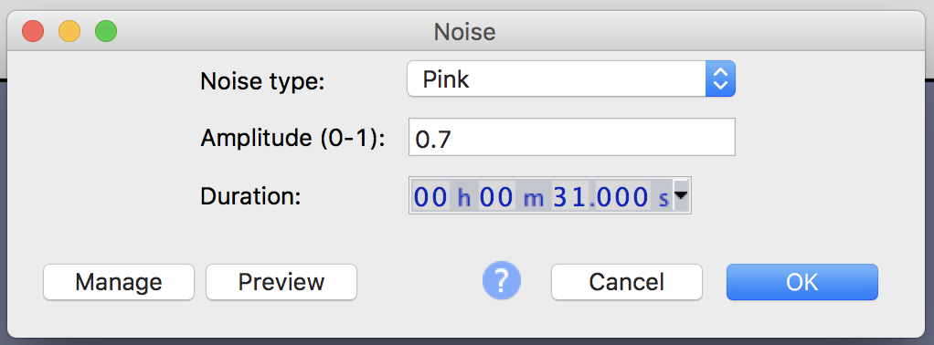
After selecting Generate > Noise… choose “Pink Noise” (of course you may choose White or Brown noise). Read about the differences here (link) (link). An amplitude of about 0.7 will work for pink noise as this will help keep the loudness units of the track in the correct range for streaming services. Read about LUFS here (link).

Choose the length to be between 30 and 40 seconds. We’ll want to choose the length to be ABOVE 30 seconds as streaming services (like Spotify and Amazon) only consider a “play” if thirty seconds of the track has been streamed. If you want your music to have “plays,” the tracks need to be longer than 30 seconds (footnote 1).

Figure 2. Noise generator settings in Audacity.
Figure 3. Track after generating pink noise.

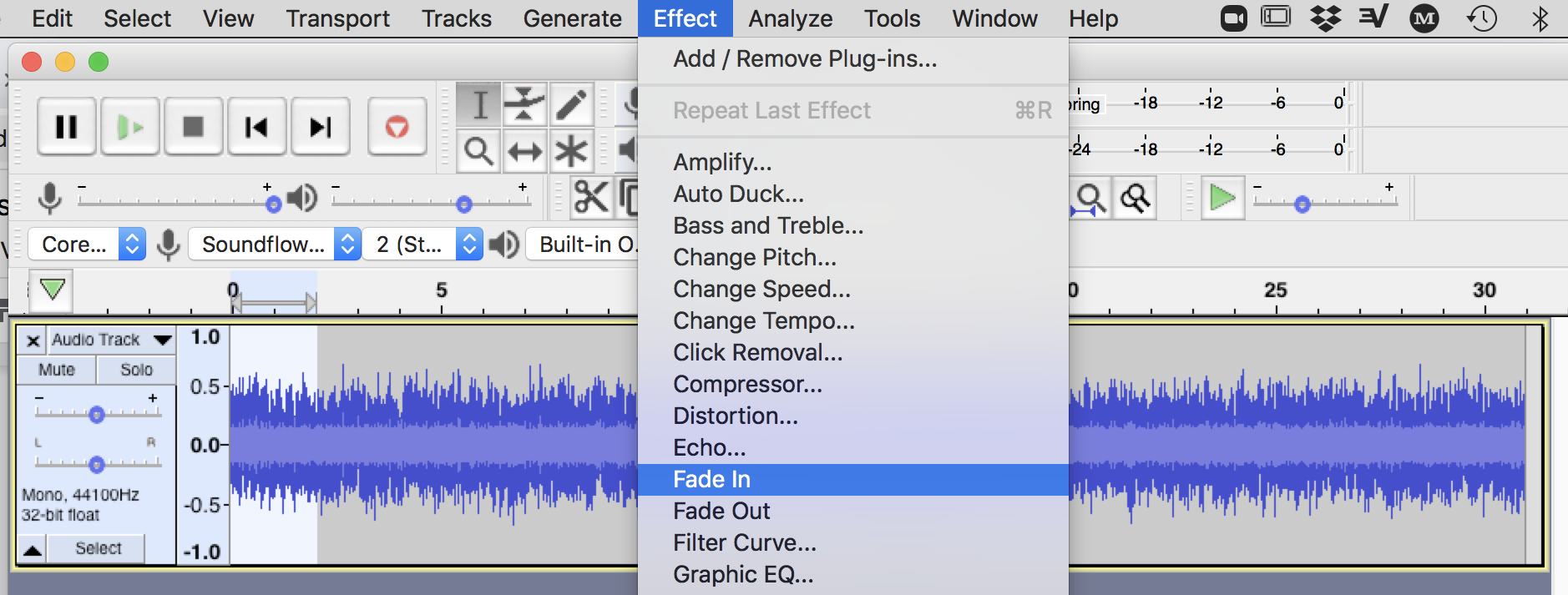
Next, we’ll need to add in fade-ins and outs. Without adding fades, at least one fade at the end, some digital distribution services (and ultimately some streaming service providers) will not accept the track as they do not allow hard ends to tracks. (note: if you are specifically creating a loopable track, then you should add “Loopable (No Fade)” to the track title to help get around this hard-cut moderation flag).

Figure 4. Add two-second fade-in in Audacity using Effect menu
Figure 5. Add two-second fade-out in Audacity using Effect menu

Export the track as .wav files 16-bit, 44.1k file. You may consider the export of the audio file as our “mixdown.” (Note: While some distribution services allow higher-quality tracks for import, our track settings get us close to our target output for this release). We are near finishing up our track, but we aren’t done. We should first listen to the audio file and then we may still want to “master” the track, or at the very least check out our loudness units (LUFS) relative to our target (streaming services) before preparing the file for distribution (footnote 2).

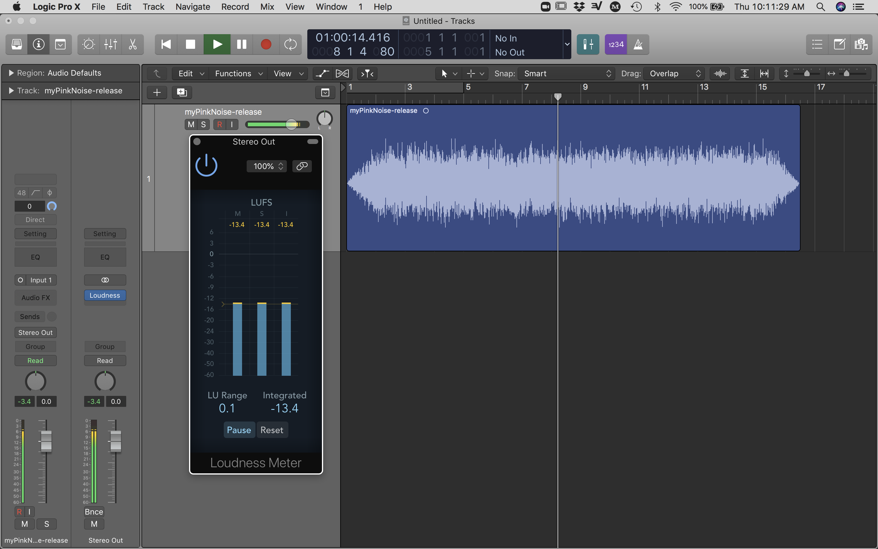
We can accomplish metering our track by opening our file inside any software that can meter LUFS and possibly control gain. If you need a free LUFS meter to quickly assess integrated LUFS, try Orban (url). Using Logic Pro X, I dragged and dropped the audio file onto the track and inserted a stock “Loudness Meter” plugin on the stereo buss. Playing back the track, the short-term and integrated meters are roughly -13.4dB LUFS. Since most streaming services use Integrated LUFS to alter the volume of tracks, a good range for most services is between -12 and -16dB LUFS. At the time of writing this, Spotify uses -14dB LUFS. (url)  You may choose to alter the gain for the track or keep what you have. Since pink noise is already “mastered” in the production sense that it has equal energy per octave, I am choosing to not add any EQ, compression, or limiting, and I will instead stick with -13.4dB LUFS on my output meter.

Figure 6. Loudness Meter, measuring short-term and integrated LUFS.

If you did happen to alter the gain, you will either want to export out the “mastered” version as .wav or .aiff from your audio software or revisit Audacity to re-export another “mixdown” at a lower volume. Again, you will want to export out audio using uncompressed audio file formats (.wav or .aif), at least until you are ready to deliver to the distribution service.

2. GENERATE ALL MATERIALS ASSOCIATED WITH THE RELEASE

The materials for a release with a distributor include:

  1. Audio file in the correct format (FLAC, .wav, .mp3, etc) and output target volume (e.g., -14dB LUFS)
  2. Cover art for the single/EP/album
  3. Track title
  4. Artist name
  5. Album/EP title (if necessary)
  6. Choose a Genre (to categorize the music)
  7. Label name (if any)

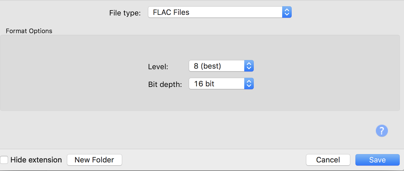
While we created a “mastered” version of the audio to be released, the target format may need to be altered before distribution. Services like CDBaby allow for uncompressed formats like .wav but others like RouteNote only take .flac or .mp3 file formats. Since FLAC is an uncompressed format and the distribution service for this walkthrough is RouteNote, let’s convert our “master” into a .flac file. Audacity software handles exporting out to this format. Just open up your mastered track in Audacity and export audio out as FLAC (footnote 3).

Figure 7. FLAC settings in the Export Audio window in Audacity software

Note: you do not want to convert to .mp3 for your release as this not only reduces the quality, but may introduce short bits of silence (10-20ms) at the beginning and end of your audio track(s). So for the case of “Loopable (No Fade)” tracks, .mp3 conversion can actually print silence into the track and cause a quick burst of amplitude rupture on streaming services due to the added silence from the codec compression conversion. This has nothing to do with buffering.

The cover art doesn’t need to be fancy, it just needs to fit the specifications. At the time of this writing, RouteNote has an image database that’s free to use and a photo resizer. If you want to make your own, RouteNote requires 3000×3000 pixel .jpg files. Just find your favorite pink color (RGB or Hex color) and fill a 3000×3000 pixel canvas with this color. I use Adobe Photoshop, but any free image editing software will do. Most other distributors also have free tools you may use to generate cover art. And should you choose to add images as part of your cover art, make sure you have permission first (again RouteNote has a free image database).

Figure 8. Color cover art (what I didn’t use but this image is 3000x3000 pixels!)
Figure 8. Color cover art (what I didn’t use but this image is 3000×3000 pixels!)
Figure 9. My 8-minute cover art for the release made in Photoshop

For this walkthrough, naming may be the hardest part. Maybe? Did I prime you to overthink it? Come up with an artist name and a track title. Just relax and let the word association flow. Seriously. Track titles can be anything— scientific “Equal Amplitude Per Octave”; direct “Pink Noise with fades”; spiritual “Soothing Pink Noise”; or cheeky, “Pink Panther’s Pink Noise”. The point is to pick a title and move on. The walk-through is about getting comfortable with the process, not to get bogged down by the details— that is, a “perfect” name. Sidenote: you cannot use “Untitled” or “No name” as these generic titles can be flagged by the distributor. You should do a quick word association for the artist name as well… remember, you never have to use your artist name again, but you must pick a name. 

Afterward, you should get on a streaming service (here) (here) or (here) and do a quick check to make sure your new artist’s name doesn’t match existing artists (unique names make searching easier, and your work/streams will be attributed to you without added hassle).  

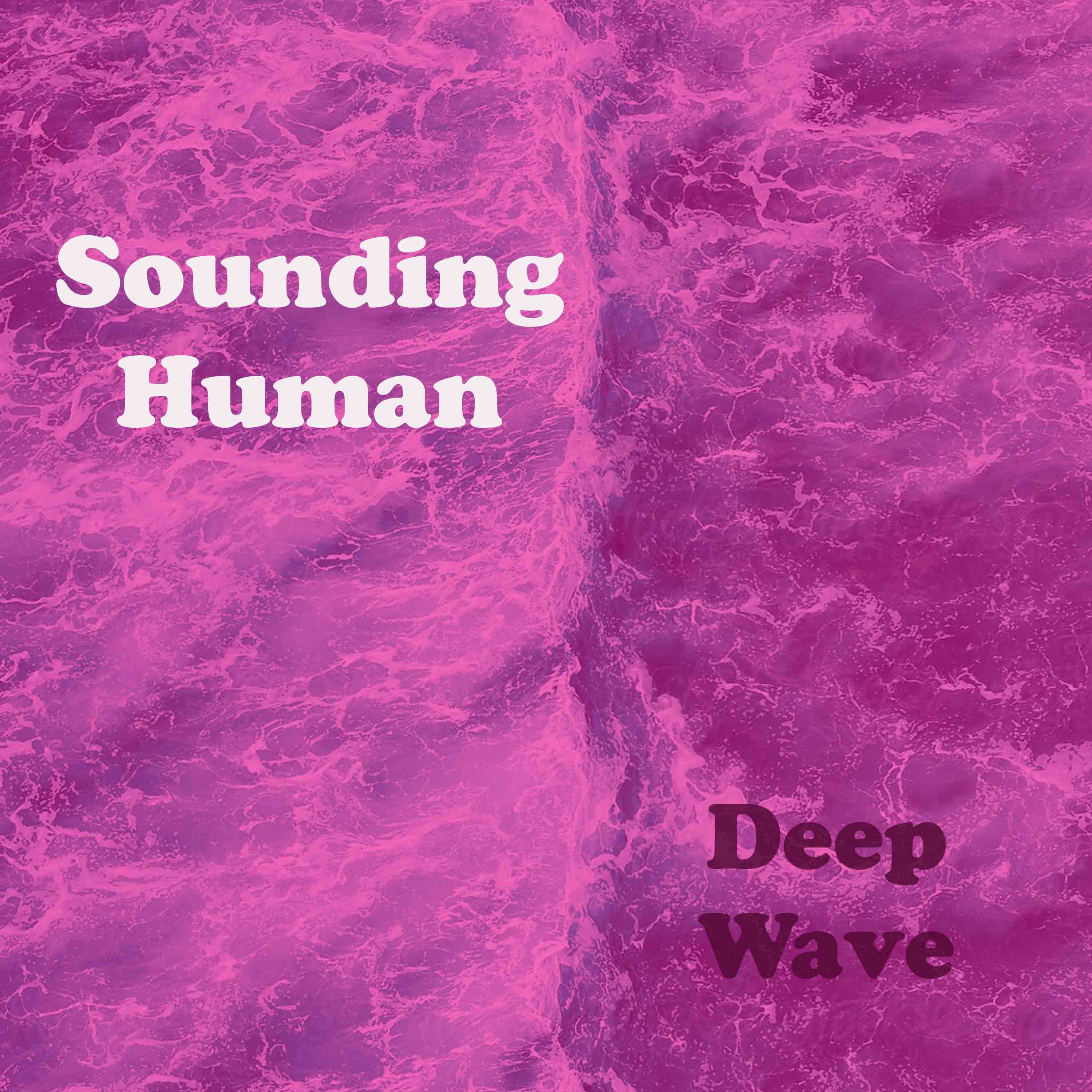
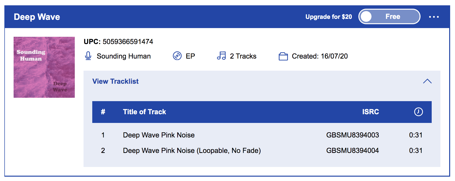
Here’s what I came up with for my track (ie. You shouldn’t use. Now on Spotify)

Artist: Sounding Human
Album/EP title: “Deep Wave” EP (can also be same name as your track)
Track 1: “Deep Wave Pink Noise” and
Track 2: “Deep Wave Pink Noise (Loopable, No Fade)” 

Ready to move on?  What? No?!  Seriously? You don’t have a name yet? Use the letters from your name in this anagram maker. (url) Take one of the top five that appears. This is your artist name.

3. REGISTER WITH ROUTENOTE DISTRIBUTION SERVICE

Register with RouteNote. (url) On the RouteNote page, click on the “Join RouteNote” button. All you need is your email and a username. If you have an account already, just log in (footnote 4).

For any release, you have to pick a distribution service (DistoKid, RouteNote, CDBaby, Mondotunes, ReverbNation, Landr, Awal, Fresh Tunes, Tunecore, Chorus Music, Symphonic, etc). You don’t have to choose the same service in each release, but you cannot release the same music on multiple digital distribution providers. I’ve chosen RouteNote as it’s free to release, will keep your music up after you release, and satisfies the purposes of this walkthrough. Fun fact: you also can share revenue with this service. Please note that all distribution services take some sort of cut, whether upfront in fees, or later on in streaming. You always retain the rights to your music. For a full list comparing all the services check out Ari’s Take (url).

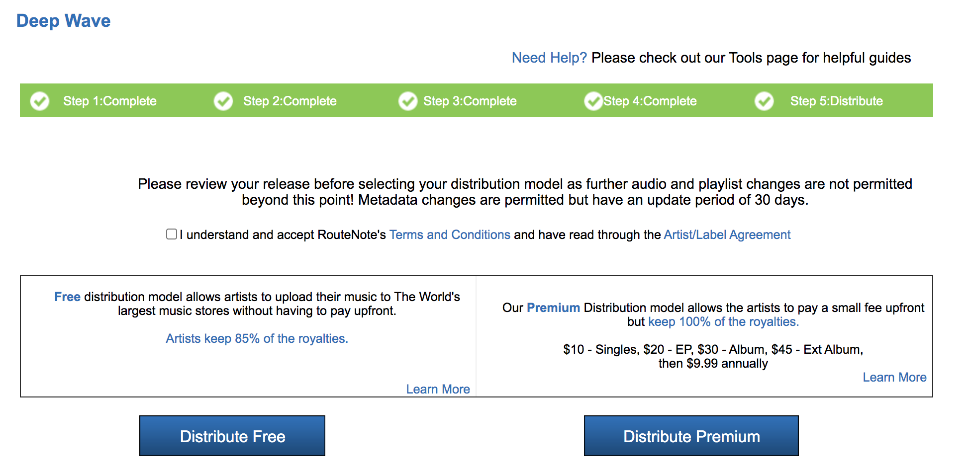
4. DISTRIBUTE YOUR WORK 

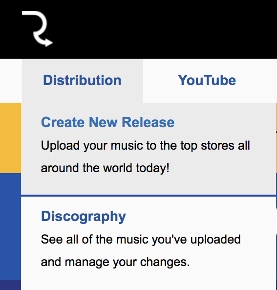
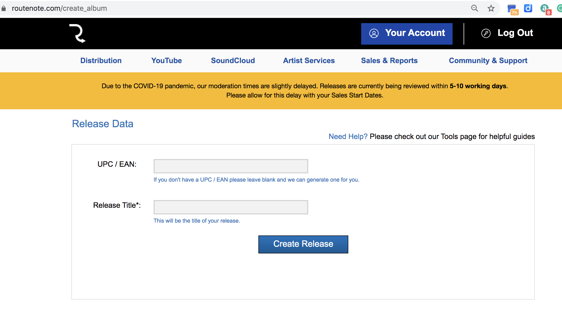
Ok. You’re ready to create your release with the distributor. Just log in to RouteNote and click Distribution > Create Release.

Figure 10. RouteNote Distribution menu

You’ll need to add your track title (or EP or Album title) to the release. Don’t worry about the UPC as RouteNote assigns you one for free. A UPC is a universal product code associated with the release. Think of it like a barcode that you see on a CD or LP. The UPC is specific to YOUR single/EP/album. Some services, like CDBaby, charge for this. It’s free here.

Figure 11. RouteNote initial Release Data input fields

After the initial title name and receiving a UPC, there’s a four-step process to the release that we have prepped for in step 2.

Figure 12. RouteNote Release overview (four steps)

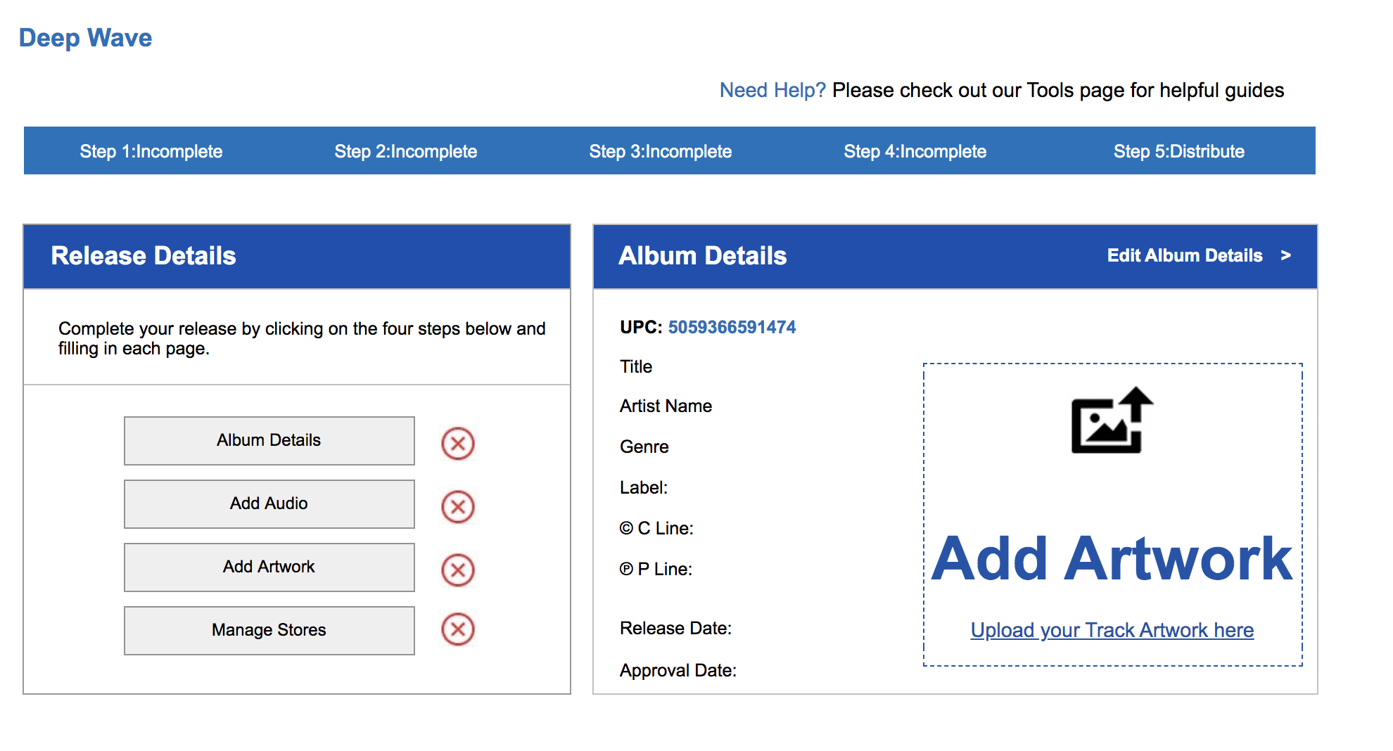
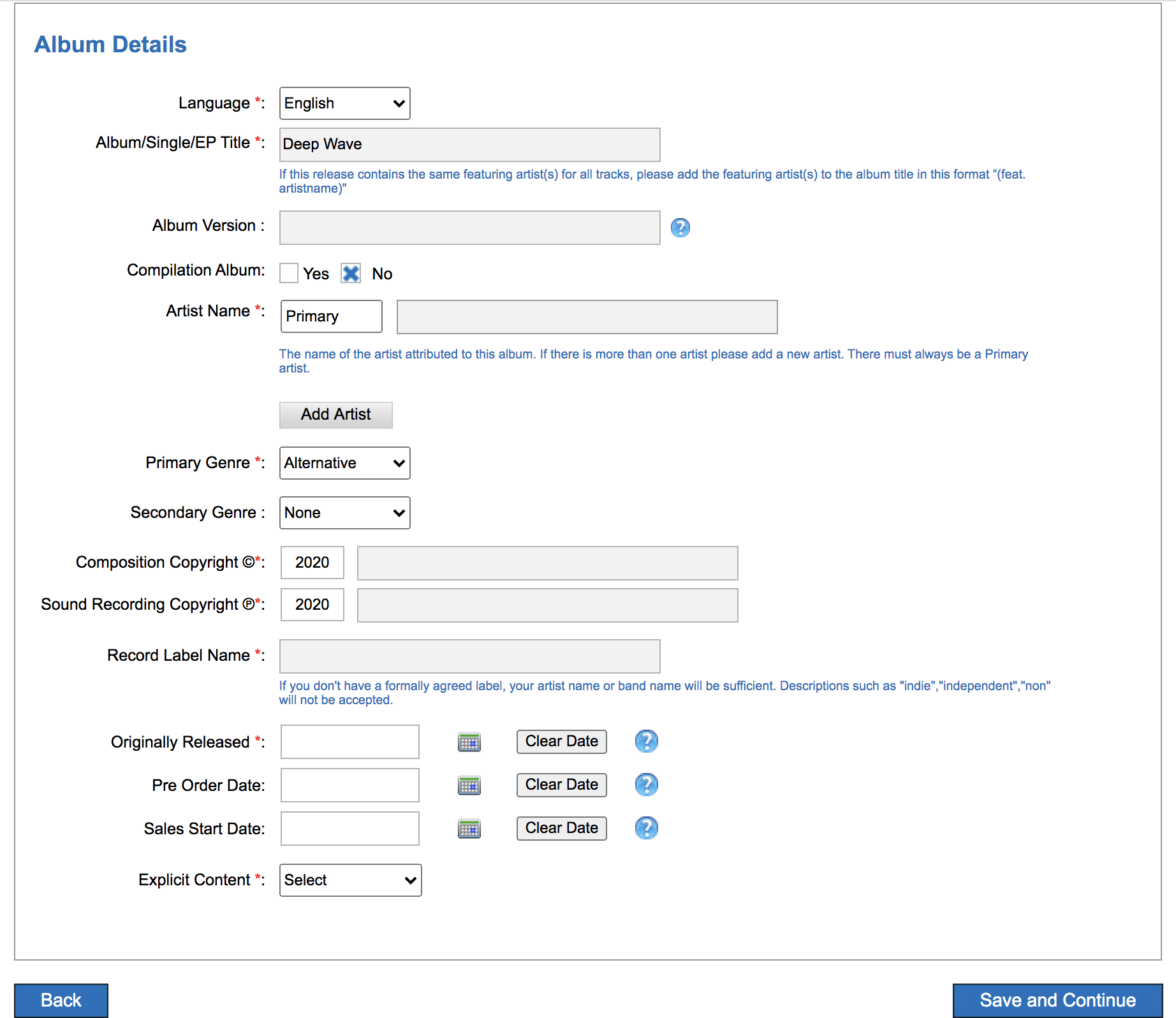
1. Album Details. See the image below for all fields. You may choose to use your own name for C and P copyright, although you may use the artist name. C is for the underlying composition (the written music) and P is for the recording (what the artist records). Often, the C and P lines on the record are attributed to the record label (e.g., Sub Pop, Matador), but not always. You’ll also need a genre, but for something like pink noise, maybe “Easy Listening”? A note about release date. If you are setting this up for music release, you’ll want to time this in advance and have an album release strategy.  As Bobby Schenk, digital marketing manager for Dub-Stuy records, puts it, “Include the 7-10 day delay in your release strategy. Release earlier rather than later with a scheduled release, as you’ll need to align with your PR machine.”

Figure 13. RouteNote Album details screen

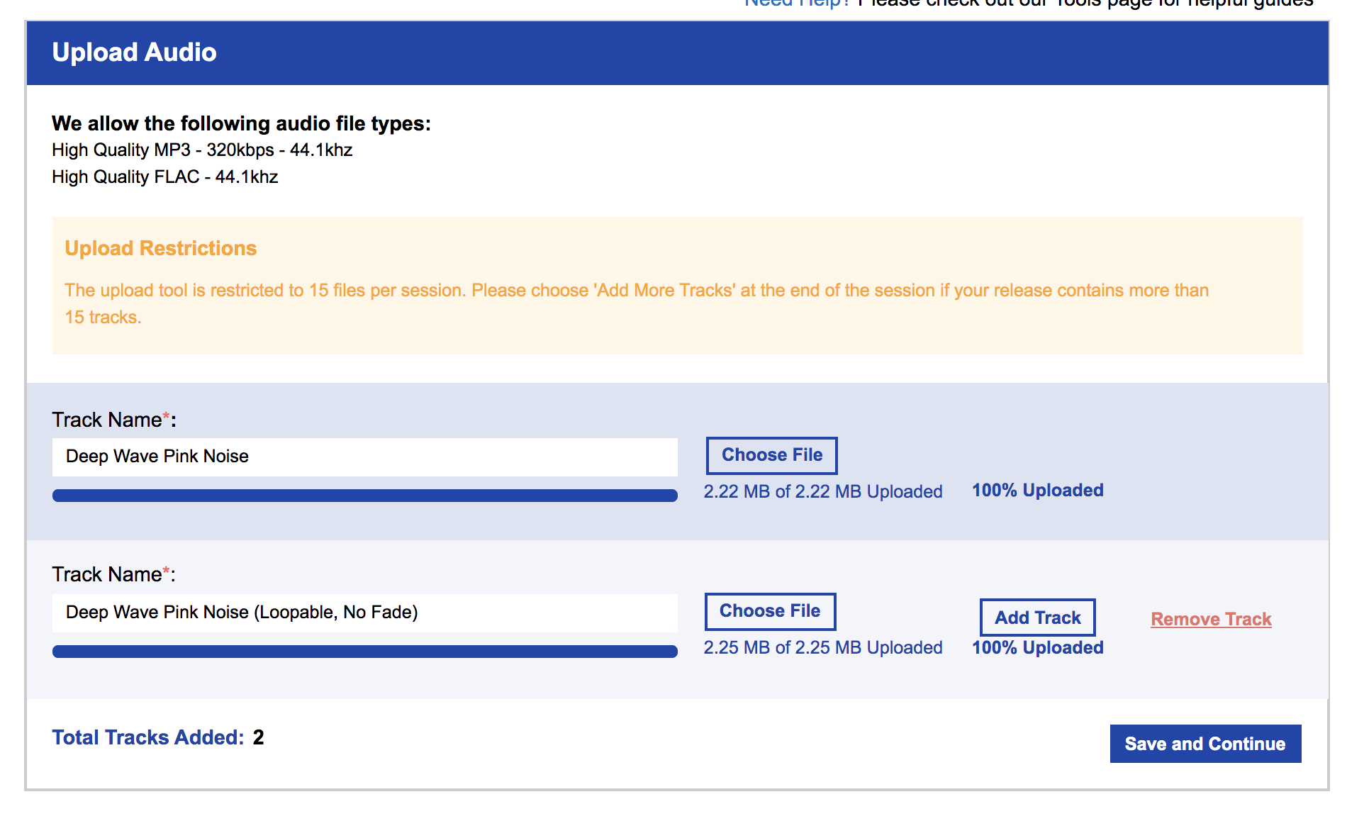
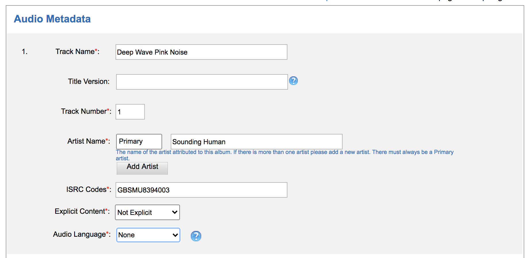
2. Add Audio. This is where you’ll upload ALL audio files. You’ll need the track name, but you’ll be asked to assign some additional metadata to each track (if you’re uploading more than one track). Since the track is pink noise with no lyrics, there will be no language associated with the track. Your track will be assigned an ISRC (‘International Standard Recording Code’) and that ISRC is attached to the recording, not the underlying composition. ISRCs are one important way for tracking streams (read royalties) as they are individual barcodes to the musical recordings. Read about ISRC (url). Read more on composition vs recording (url).

Figure 14. RouteNote Upload Track screen
Figure 15. RouteNote Track Metadata screen

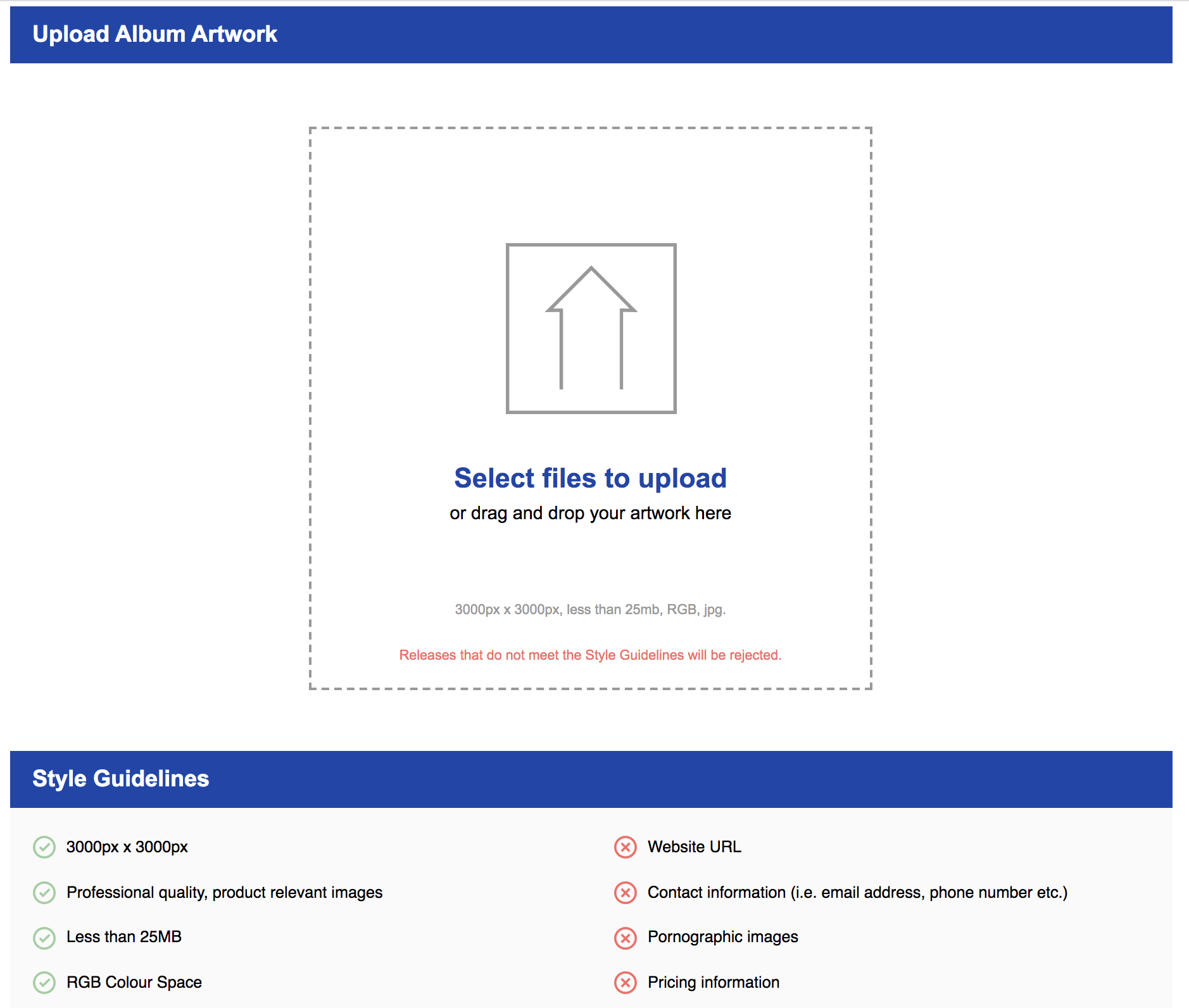
3. Add Artwork. We’re halfway there! Next, we need to upload our album/single cover art. Remember, the guidelines are hi-resolution files, and for RouteNote that is 3000×3000 jpg files only.

Figure 16. Route Upload artwork Screen

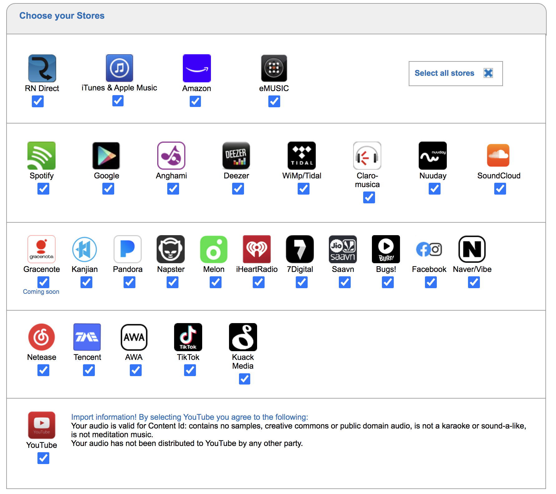
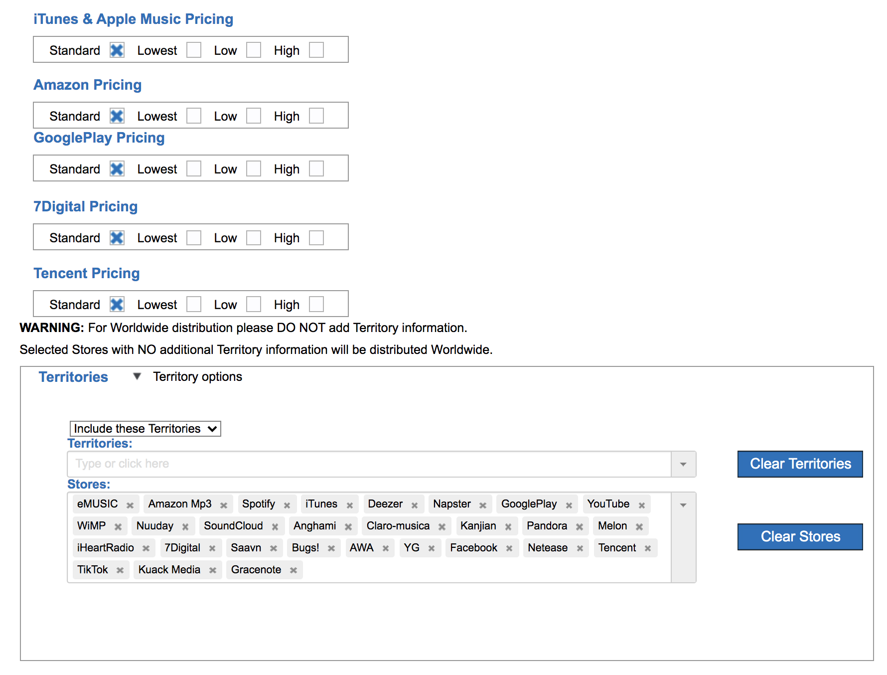
4. Choose Your Stores. This part should be simple. What services do you want your music on? Spotify? YouTube? Tidal? All?  You can be picky but often the default is to distribute on all platforms all over the world. RouteNote makes it easy with one button-click.

Figure 17. RouteNote Store selection screen
Figure 18. RouteNote Territories selection screen

Now you’re ready to distribute! All you need to do is check over your work and then click on “Distribute Free.” And that’s it! RouteNote will take a cut of your streams (15%) but there are no upfront costs to the process.

Figure 19. RouteNote Completion Screen. Two options for distribution (free vs paid).
Figure 20. RouteNote Post-Distribution. In Review details

5. NOW WHAT?

The release will take about a week or so to be released, at which point you should receive an email. If there are issues with your work (track titles too generic, audio file has copyright issues, etc.) you will receive an email in which you’ll need to resolve all issues before the release can move forward (footnote 5). 

While you wait for your release to go through moderation, here are a few things you’ll want to consider as part of any release that you do in the future. Maybe not part of this walkthrough, but certainly if you are getting serious about releasing your music.

1. Check out new music. Listen to the walkthrough release, Sounding Human, on Spotify, 🙂

 https://open.spotify.com/album/2qUZchgXBIWkz7Di6jdFiY?si=_2LF9vwmTICyeSXMCzATTg 

2. Register your work(s) with a Performing Rights Organization (PRO)

If you’re not already part of a PRO (ie., ASCAP, BMI) you should strongly consider it. …. You’ll need to be registered with a PRO in order to register your work for admin publishing royalties among other things. Here’s some reading about PROs (url) (url). Quick note: A composition can have multiple recordings (ISRCs), but only one composition (ISWC). What’s an ISWC? Read here (URL).

3. Register your work on SoundExchange

At this point, your music will appear on streaming platforms that have two types of plays (interactive and non-interactive). Interactive streams are where people hit the play button on your music (or if it’s on a playlist. However, digital distribution services like RouteNote cannot collect on non-interactive streams (radio-type play). SoundExchange (url) is the collector of these royalties. Registration is free, but you’ll need to upload and claim all your recordings if you want to collect within this market. Want to learn more about this? Read here (URL)

4. Claim your Artist Profile 

After your release is live, you’ll want to decide if you want to claim your artist profile. Doing so allows you to update profile pic, add a bio, create artist playlists, and even track who is listening to your music every day. Claim your artist on Apple (url), Spotify (url), Amazon (URL).

5. Start a Digital Store

Some services offer you to sell your music directly to fans/consumers, but many are not digital stores. In this case, you may consider a digital store like Bandcamp (url), where you can sell your music as direct downloads, all from one location.

That’s basically it! In one hour or one pot of coffee (hopefully that’s all it took), you’ve gone from zero to release. If you dug this walkthrough, please share, follow my music on Spotify (url), and pay it forward in your own musical community. Thanks for being an active participant!


Footnotes:
1. 30 seconds for a stream count seems to be an agreed-upon time length. I ran a test on my EP Software 1.17 (Spotify link) with the final track clocking in at 26 seconds. After a year and with friends streaming this track across multiple services, the track still has 0 plays for royalties. If you want to dig deeper on Spotify’s algorithm, which helps support the 30-second rule, check out this article (url).

2. Streaming services typically average -12dB to -16dB Integrated LUFS (loudness units to full scale). All streaming services use LUFS to act as your own personal DJ, helping adjust the volume between tracks that may be coming from a different genre, era, or artist. It’s become more common that Spotify uses -14dB LUFS for its target. This means you that if you crush your track with an integrated LUFS (overall average loudness) of -8dB, Spotify can very well turn your track down by -6dB making it half as loud… meaning you lose all that intensity you spent so hard to work for. Use a meter! (url)

3. Make sure you always listen to your work after you export it! You want to make sure everything sounds correct before you upload your audio file. Do NOT distribute without listening to your final work first.

4. RouteNote registration full disclosure. I included a referral link for registering with RouteNote in step 3. Referral ID: 2f79120f. You get your full cut regardless; RouteNote simply takes a percentage of their own earnings and passes it on to me. Thank you for supporting articles like this with using the referral code.

5. Note for our walkthrough that releasing a noise track via RouteNote will not appear on Apple Music / iTunes. I inquired with RouteNote directly, and here’s what their moderation team had to say (email dated 7/24/2020), “Unfortunately iTunes no longer accept white noise/nature sounds content due to the high amount that was being uploaded to them. They have asked us to no longer send it to them, for this reason the store was blocked.” If you go through a different distribution service, you can get noise albums on Apple Music (case in point, here’s an album I created for an Oregon-based birth center: https://music.apple.com/us/album/calming-sounds-for-pregnancy-birth-and-parenting/1522834278)

Challenge Song: Supertramp “The Logical Song”

The students in my Audio Recording Techniques III (Spring 2019) course at University of Oregon had ten weeks to recreate a recorded song of their choice. They voted on reverse engineering Supertramp’s “The Logical Song” from the band’s 1979 album, Breakfast in America. The goal was to get the song as close as they could to the original recording. They recorded, overdubbed, mixed, mastered, and played parts!, on all elements of the song. I am amazed at their accomplished product. Enjoy!

Kyma: Encapsulation

While teaching Data Sonification at the University of Oregon, we talked a lot about inference preservation, communication of idea, filtering and bias of data, and by extension, tool building as a process for supporting sonic hypotheses. To that end, I wanted to empower students with their own work inside Kyma, so we spent a class walking through the process of Encapsulation.

Encapsulation allows one to take a Sound and “create a simpler, cleaner interface for that Sound by reducing the number of controls and putting them all on the same level. Encapsulating a Sound does not make it more computationally efficient, but it does present a clearer control interface between you and the Sound” (Kyma X Revealed 2004: 293). Or, another computer music way to say it…
Max/MSP::abstraction
Kyma::encapsulation

For those familiar with NeverEngine Labs, one can understand the power of encapsulation to create some really great Sounds that serve compositional, sonic, aesthetic, and educational goals. Encapsulated Sounds can help one save time, grow as a practitioner, and engage with the growing Kyma community. Tool building and sharing also invites positive activities like research, collaboration, and publication. The Kyma X Revealed section on Encapsulation (pp. 293-303) is a great starter, but can be a difficult first reference for the uninitiated. This article seeks to provide a current walkthrough of encapsulation that supplements existing documentation.

What will you need? Head over to the Kyma Community Library (https://kyma.symbolicsound.com/library/encapsulation-walkthrough/) to grab walkthrough files, but beyond this article, you will find Kyma X Revealed (293-303), any software to create a .png icon (e.g. Adobe Illustrator, Photoshop), and your design thinking hat helpful.

The process to Encapsulation follows five basic steps.
1. Create a Sound(s) to encapsulate
2. Define your controls and change the values (numbers or !EventVariables) to ?vars
3. Create a new class (Action > “New class from example”)
4. Add default values to the controls to open up Class Editor
5. Add descriptions and icon, set parameter types, and close to Save Class.

Step 1. I created a simple Sound to encapsulate (Figure 1).

Figure 1. Kyma Sound, a one-sample wide impulse of N-samples long, ready for Encapsulation.

The Kyma Sound to encapsulate, a one-sample wide impulse of N-samples long, is meant for controlling the amplitude of a single band in a spectral analysis of the same sample length (e.g. 256 samples). Bearing this user case in mind, where the encapsulated Sound will effect a spectral analysis’ amplitudes, Figures 2 and 3 depict the parameters fields of the two Sounds that create the effect (SyntheticSpectrumFromArray and DelayWithFeedback, respectively).

Figure 2. SyntheticSpectrumFromArray Sound parameters ready for encapsulation.
Figure 3. DelayWithFeedback Sound parameters ready for encapsulation

Step 2. I labelled the most helpful controls for the encapsulation process as green ?variables (Figure 2 and 3). Green ?variables are what enable a user to access parameter fields after encapsulation. The three user parameters, ?ImpulseAmplitude, ?samples, and ?Delay provide the user with the ability to control the amplitude of any single partial in a spectral analysis of n-window size. SyntheticSpectrumFromArray (Figure 2) creates a n-sample long spectrum with only one envelope. Since Kyma handles spectrums in the time domain as Amplitudes in the Left channel and Frequencies in the Right Channel, we treat the Partials parameter field more like the Sample length of the analysis. A single envelope is generated with the Envelope parameter field set to 1, there will only be one partial to control, with all other envelope amplitudes set to 0. That single envelope’s gain is controlled by ?ImpulseAmplitude. The Left Channel is selected, which means the SyntheticSpectrum Sound will only impact the spectrum partial’s amplitude, not its frequency. [See Gustav Scholda’s in-depth video for how spectral analysis works in Kyma and how to spectrally manipulate frequency and amplitude.]

?samples is meant to match the length of the spectral analysis it will later control. The delay length is also set to the same length, as DelayWithFeedback enables the single envelope to “scrub” across the sample length. In essence, ?Delay enables a user to select which partial’s amplitude they will effect.

Footnote: An esoteric note about this particular Sound. The Amplitudes parameter field of SyntheticSpectrumFromArray expects an array. Because the variable ?ImpulseAmplitude is a green ?variable, Kyma will prompt and ask the user if the ?variable is an “Element” or an “Array.” Because the Sound is meant to control a single partial, the ?variable is an “Element,” not an “Array.”

Step 3. Time for Encapsulation. From the main menu, select Action > New class from example (Figure 4).

Figure 4. Kyma Action menu, New class from example, which encapsulates the chosen Sound.

Step 4. The menu selection will then generate a user prompt to add default values to the three green ?variables (Figure 5). All variables are “Values” and whatever is entered will generate defaults values one may alter later. For now, one may enter 1 for ?ImpulseAmplitude, 256 for ?samples, and 0 for ?Delay.

Figure 5. Green ?variables default value user prompt.

Step 5. The real encapsulation work begins adding Class name, descriptions, icon, and Input/Output type for formatting look and feel. Figures 6 and 7 depict the encapsulation editing process before and after.

Figure 6. Encapsulation editor before edits are made.
Figure 7. Encapsulation editor after edits are made.

The various fields altered for the encapsulation are as follow. Name is the name of the class, which can be searched for. Class description is the overall description, which can include overall sonic description, use cases, and user specific comments.

Parameters are designated before creating a new class. Each ?var ends up as a parameter field. For example, ?samples becomes the parameter field “Samples.” Naming a ?var sets the Class parameter field name. The parameter field in the Class editor contains our default value from the previous step, but can be changed in the editor. In addition, the Parameter options in the left tab will enable one to set Type, Field Type, and Category of the Parameter altering how the parameter field behaves and looks. Figure 7 depicts two of three parameter fields and these options.

Close the Editor window to save the class. You may always edit the class by choosing the “Edit class” option from the Action menu (Action > Edit class). Figure 8 shows the completed encapsulated sound.

Figure 8. Kyma Sound after encapsulation. Three user fields generated in the process.

Example

Figure 9 depicts our new One Sample-Wide Impulse Class played through a 256 sample-wide oscilloscope. Since the delay is set to 0.5, we see our single sample residing in the middle of the oscilloscope (128th sample). Because the single sample may be moved in time (Delay parameter) and has control of gain (ImpulseAmplitude parameter), the Class may be used as a partial picker in Spectral Analysis.

Figure 9. One Sample-Wide Impulse Class running through an Oscilloscope at full volume, with delay set to 0.5

Figure 10 depicts spectral analysis in Kyma, where amplitude and frequencies are divided between left and right channels. The first partial is displayed as the first sample, second partial as second sample, etc. Understanding this concept, we may use One Sample-Wide Impulse to control (read multiply) amplitudes of the left channel in a spectral analysis.

FIgure 10. Live Spectral Analysis (256 samples) in Kyma shown within an oscilloscope. Left channel are amplitudes, and Right channel are frequencies (multiplied by halfSampleRate)

Figure 11 shows how an encapsulated Sound is used to multiply against amplitudes of a Spectral Analysis.

Figure 11. One Sample-Wide Impulse multiplying the Amplitudes of a spectral analysis, so the Class functions as a single partial picker.

Figure 12 shows oscilloscope view of partials, with single sample wide (one partial) amplitude control. Delay is set relative (0-1) to the 256 partials in the analysis.

Figure 12. Before and After oscilloscope views of the One Sample-Wide Impulse Class multiplying the Amplitudes of a spectral analysis.

Two audio examples using Beck “Dreams” to depict the One Sample-Wide Impulse Class in use as a partial picker.

Audio 1. Beck “Dreams” running through live spectral analysis using a 256 sample window. No partial picking.

Audio 2. Beck “Dreams” with the One Sample-Wide Impulse class controlling playback of a single partial of the 256 sample live spectral analysis. Audio sweeps from a singular low partial to high partial selection and then back down again.

Samuel Pellman’s Tower of Voices

By Jon Bellona and Ben Salzman. (Note: This post is a part of a presentation with Ben Salzman at the 2018 Kyma International Sound Symposium in Santa Cruz, CA.)
[Above photo: Nancy L. Ford]

On Music faculty at Hamilton College since 1979, Samuel Pellman devoted his life to making music with students and turning them onto art. I was happily one of those students. After all, it was Sam who led me to pursue my graduate degree in Music. I’ve since earned my Music doctorate and had the opportunity to catch up with Sam at a few Kyma conferences over the past few years.

Sam was a sturdy mentor and friend, and one I knew I could bounce any idea or question off of. He was just someone I counted on being there when I could use a little help. Tragically, all that changed in November 2017 when Sam was struck and killed while out riding his bike. As previous students, Ben (H’14) and I (H’03) look back and see there is much to be gained from Sam’s work, his presence, and his joie de vivre. Sam’s ideas are woven into the sonic fabric of Kyma. Sam may have been at times quiet and his voice soft, but his work remains a powerful force in the sonic arts. His pitch design for Flight 93 National Memorial (Tower of Voices) sonically embodies the dead in a way that pushes sound to the forefront of remembrance. The National Memorial is one of the first in the country to embrace sound as its defining factor. Sam also developed digital interactive sound installations in the 80s and 90s when MIDI and digital sensors were first coming on line. And Sam’s music hoists micro-tonality and its mathematical roots of equal temperament to the aural top, creating interesting and complex structures amidst electronic synthesis techniques. We will discuss the threads in Sam’s work, especially those using Kyma, and how these threads intertwine with his ultimate work, Tower of Voices.

This webpage contains embedded links that jump to the musical or cultural reference. We encourage you to listen, click, and read along with us as we talk about Sam Pellman and his work. Feel free to skip to the bottom for videos and links.

///// Sam at the Kyma International Sound Symposium (KISS) /////

Over the last eight years, Sam presented work at KISS five times: 2010, 2012, 2014, 2015, and 2017. Sam grew up an organist; he regularly performed at the Clinton United Methodist Church and during the convocation ceremonies at Hamilton College. Yet, much of Sam’s work at Kyma conferences were interspersed with whole-number ratios and micro-tonal temperaments. Sam compositionally split the twelve divisions of the octave as much as he performed within their boundaries. For example, Sam’s various Peculiar Galaxies, which are part of his Selected Galaxies (KISS 2012; Ravello Records 7912), uses pitches “based on a dorian scale, tuned in 5-limit just-intonation, that is friendly to both quartal and tertian harmonies (i.e., harmonies built of fourths or thirds, respectively)” (Pellman 2012a; 2012b; 2012c).

The Selected Galaxies album also includes Selected Cosmos (KISS 2014), which is a two-tone sonification of human DNA (as reported by the Human Genome Project) using Kyma. Sam supports these two sequences of pitch and timbre by drone timbres, whose pitches are Shepard-filtered tones, “54 octaves above the sound emitted by an active galactic nucleus in the Perseus Cluster.” (Pellman 2015).

///// Tower of Voices /////

Sam’s ultimate work, and perhaps the one which will become his most memorable, is his pitch design for Tower of Voices. Tower of Voices is a visual and audible reminder of the heroism of the 40 passengers and crew of United Flight 93 that was hijacked and crashed in Shanksville, Pa., on Sept. 11, 2001. According to the National Park Service, “there are no other chime structures like this in the world” (NPS 2018). The Tower is 93 feet tall with 40 chimes measuring from 59 1/4″ to 97 7/16″ with walls “designed to optimize air flow… to reach the interior chime chamber” (ibid). Sam’s pitch design of the forty chimes “allows the sound produced by individual chimes to be musically compatible with the sound produced by the other chimes in the Tower. The intent is to create a set of forty tones (voices) that can connote through consonance the serenity and nobility of the site while also through dissonance recalling the event that consecrated the site” (ibid). While Sam designed the frequencies of the forty chimes, the chimes were built by Gregg Payne, an artist based in Chico, CA.

The Tower of Voices has eight columns with five chimes in each column. Sam indicated in his files preferences for particular groupings of chimes and he collected them horizontally. For tuning the chimes, Sam based his work on whole-number ratios. “The tuning ratios indicate the frequencies of the chimes relative to a middle-C of 264 hz. The chimes are tuned according to a system of just intonation, based on whole-number ratios” (Pellman 2017). Sam went through five versions of his tuning system before settling on the final system, as shown below in Table 1. Each cell in Table 1 depicts the pitch, frequency, and whole-number ratio (in relation to C=264hz) of each chime tone.

Table 1. Tower of Voices Pitch Design

C pitch
264 hz
1/1 ratio
E
330hz
5/4
E
334
81/64
F#
372
45/32
G
396
3/2
B
495
15/8
B
501
243/128
C
528
2/1
D
149
9/16
G
198
3/4
D
293
10/9
D
297
9/8
E
330
5/4
F#
367
25/18
F#
372
45/32
G
396
3/2
G
198
3/4
E
330
5/4
E
334
81/64
F#
372
9/8
G
396
3/2
B
495
15/8
B
501
243/128
C
528
2/1
C
264
1/1
D
297
9/8
E
330
5/4
E
334
81/64
G
396
3/2
B
495
15/8
C
528
2/1
C
535
81/40
C
264
1/1
C
267
81/80
D
293
10/9
E
330
5/4
E
334
81/64
F#
367
25/18
F#
372
45/32
G
396
3/2

Sam created several sonic prototypes/models throughout the build. Aluminum chimes were recorded in Tuzigoot, AZ, which Sam then used for modeling the sound of the forty chimes. One of the most striking auralizations is his October 2016 prototype built using Kyma, and which is still available on the National Park Service website for Tower of Voices. That same prototype can also be heard below.

Inside Kyma, Sam used multiple Sample Sounds played through a single MIDIVoice object that was triggered using a custom Max/MSP patch (sending MIDI note on/off messages). Sam’s model uses a lot of memory, and his Kyma’s Multigrid model is only able to playback on a Paca(rana). To optimize playback on just a Paca, we leveraged the MIDIVoice Sound script, and in turn, we were able to keep all the ratios in a single script array, referencing a single 264hz audio sample.

While the Tower of Voices model doesn’t represent Sam’s final pitch design, Sam did create a final auralization before his death based on his final v05.1 tuning design. For his aural model, Sam relied on a custom Max/MSP patch playing back buffers of five audio files at various speeds (read frequencies). The model runs by generating random timing bangs, where each bang selects a new number from a Coll object (an array list of pitch ratios and audio file names). The output of the Coll object first selects the appropriate audio sample to playback and then alters the sample playback speed based upon the pitch ratio. A final bang plays back the audio file. The use of a poly~ object in the patch allows multiple chimes to be played back simultaneously.

Sam never made a Kyma version of his latest tuning design, and since one can hear digital artifacts in the Max/MSP model, we decided to merge Sam’s tuning design inside Kyma. We wanted to hear the tuning design with the same high fidelity that Kyma delivers. Using our optimized Kyma Sound of a single MIDIVoice Sound script, we took Sam’s v05.1 tuning design and input these ratios into the script’s pitch array. The result is all at once beautiful and all Sam. We recorded a short bit of Sam’s final tuning design using Kyma, which can be heard in the audio player immediately below.

Sam’s compositional work is a by-product of his tireless passion for students and ideas, collaborative learning and theoretical concepts, and the intersection of science and the arts. Sam’s upbeat ethics, positive attitude, and dedication to the hope and optimism of the arts to construct meaningful dialogue has helped create a catalog of meaningful works. We know Sam will live on in the memory of the Tower of Voices, where each and every time a chime is rung remembering those who lost their lives on Flight 93, his ideas sound out across the valley of Shanksville, PA.

///// More About Sam /////

Sam Pellman studied with David Cope, Karel Husa, and Robert Palmer.  Sam was co-director of the Studio for Transmedia Arts and Related Studies at Hamilton College and oversaw the development of Hamilton’s multi-million dollar Kennedy Center for Theatre and the Studio Arts. Sam served as Associate Dean of the Faculty, Posse mentor, and was recipient of Hamilton College’s 2015 Alumni Association’s Distinguished Service Award. Sam’s work can be heard on Innova and Ravello Record labels, and found at: http://academics.hamilton.edu/music/spellman/MfS/MfS.htm

///// Selections of Sam’s work /////


Peculiar Galaxies: UGC4881 from Samuel Pellman.


KISS2014 — Selected Cosmos: Sounds of Life, Samuel Pellman from Symbolic Sound.

///// References /////

///// Additional Links /////

Challenge Song: Massive Attack “Teardrop”

The students in my Audio Recording Techniques III (Spring 2018) course at University of Oregon had ten weeks to select and recreate a recorded song of their choice. They voted on producing a recreation of Massive Attack’s “Teardrop.” The goal was to get the song as close as they could to the original recording. They recorded (and played parts!), mixed, and mastered all elements of the song in just under ten weeks. I am so proud of my students and what they were able to do. I am posting here to give me (and I hope you!) a smile when one needs it.

Max/MSP Package: Korg Nano

Ever since Cycling 74 introduced the idea of packages in Max 6.1, I’ve been pretty excited. Previously, there wasn’t a great way to distribute and install tools, objects, externals, media. And if you wanted to use anyone else’s tools, you had to wade through the murky collection of application directories and dump in single files–an unfailing way to ensure that you’d have to re-install these tools after a Max/MSP update.

With packages, Cycling 74 got rid of the mess. Tool creation, installation, and for me, distribution is clear and simple. Even if I’m developing my own set of abstractions for nobody’s computer but my own, packages provide a platform for a confident working-practice with long-term benefits. This post is meant to outline the pros of Max packages by walking through a working example of how one can set up her/his own Max package.

While I have created several Max packages since 2014, the post will outline my latest Max package, Korg Nano.  It’s a basic example, two objects that comprise a software implementation of the Korg nanoKontrol USB controller, certainly enough to get one started.

Installation
After downloading the Korg Nano package, unzip the file and place the unzipped folder directly into the ‘packages’ directory.  For Mac users, the folder is Applications > Max 6.1 > packages.  Or, you can read a short article by Cycling 74 on packages for installation.

What It Is
In short, packages provide global access. Autocompletion, media in global search paths, extras in the top Extras dropdown menu, option clicking helpfiles, it’s all there. What the Korg Nano package provides is a software listener for the 151 controls on the Korg nanoKontrol USB controller. The package is meant to be a plug ‘n play solution for this hardware device (and I use it for prototyping all the time).

After installation of Korg Nano in the Max packages directory (make sure you restart Max), navigate to the folder.  You will see four folders inside (docs, help, media, patchers) and a README file. Each folder has a unique purpose, and there are many more one can add (extras, javascript, clippings, templates, etc). If you’re curious, there is an “about packages.txt” file in the packages directory that outlines the finer points of Max packages. For now, we’ll unpack these four folders (docs, help, media, patchers).

Max/MSP Autocomplete feature for Korg Nano package.

The patchers folder is where you throw your abstractions and objects (not externals), including any additional bpatchers that you may have used to create your objects. Of course, if your package depends upon third-party objects, you can place them here (and within any named subfolder). For Korg Nano, there are two main objects, korgnano and korgnano.inputmenu.  korgnano is built from several bpatchers, which one will see listed in a subfolder (“patchers > korg_nanoKontrol”).

The media folder allows one to place images, audio, and video. This folder becomes global (after restarting Max), so you can also use packages as a way to manage media instead of worrying about “filepath” when you move from computer to computer. Since Korg Nano is a software implementation of the USB hardware controller, I used image buttons that simulate the look and feel of the hardware controller. Placing images in the media folder ensures they will be found, regardless of what computer I am using.

The help folder is exactly what one would expect. Help files ending with the extension .maxhelp.  While help files are useful (e.g. option-click an object to access its help file), Max packages allows one to provide some serious help to the help files. This helpful power boost comes by way of the docs folder.

Korg Nano help file that looks like a standard Max help file.

The docs folder contains reference files that enable hover tooltips, documentation window text, uniform descriptions, and fancy descriptive break downs and object links from within the reference window. To understand what is happening in the help file screenshot above, let’s dig into the docs folder.  Navigate to the “korgnano-0.0.1 > docs > refpages > korgnano > korgnano.inputmenu.maxref.xml” file.  This xml file contains all the descriptions that get pulled for the help file. While this file contains confusing html/xml style tags, one need only look to two examples to see their power.

The first example comes from the first two xml tags <digest> and <description>.  These two description tags show up in the Autocomplete menu, the documentation window, the reference window (outside any help file), and the help file’s title object (actually, a jsui object that uses an application Max script “helpdetails.js” to parse these xml tags and display them for clean documentation).

The second example of documentation power comes from the <seealsolist> tag near the bottom of the .xml file.  One only needs to place additional object names here (e.g. “<seealso name=’korgnano’/>”) and links automatically appear in the reference documentation window, linking to your objects’ help files. This is handy here, as I want to link the korgnano object and the korgnano.inputmenu object together since these objects are symbiotic. The korgnano object grabs data from your Korg hardware controller and then sends the controller data direct to korgnano.inputmenu objects.

Docs, Help, Media, Patchers. That’s it.  A Max package that enables software listening for the Korg nanoKontrol, neatly bundled for distribution. Clear documentation files to help anyone navigate the tools, even me! when I revisit my tool a few months down the line. However, I do not need to distribute to reap the benefits.  Clippings, templates, patchers, or even externals that I use often in my own work have a place within a Max package, easily searchable and documented so I have a working practice that is efficient and scalable. For anyone working in Max, packages offer a clean way to keep your sh** together.

Korgnano object help file


Reference
Korg Nano Max package

Notes
Packages also work with Max 7. While my example was built using Max 6.1, there is no reason why it shouldn’t work in Max 7. Email me if you have issues.

Speaking of issues… if you’re having trouble with autocomplete, try creating a message object in a Max window with the text “; max db.reset”.  This will refresh Max’s preferences, but may take 60 seconds+ to reload. Here’s the original forum post where I found this fix.

Photoresistor Theremin

Tired of software, longing for the touch and feel of circuits, I’ve been looking for something to satiate my sonic hunger. And, I wanted to get my hands dirty. So, I placed a small order of electronic parts with mouser.com. Additionally, ever since having discovered that the cigar store in Staunton, VA sells nice wooden cigar boxes between $3 and $5 (size and quality), I’ve been itching to put a nice piece of analog circuitry inside.

Thanks to Nic Collins (Handmade Electronic Music: The Art of Hardware Hacking p.161), I found a nice schematic on controlling pitch and volume with photo-resistors. (note: instead of throwing up the schematic as an image, I have posted a pic of my breadboard circuit based upon his schematic below. Regardless, I urge you to support Nic by buying his book. It’s really good).

After wiring the circuit up on a bread-board, I noticed how quiet the theremin sounded. To boost the signal, I needed an audio amplifier, so I turned to the good, old Radioshack project book, Timer Op Amp and Optoelectronic Circuits and Projects Vol. 1 (p.43). Forrest Mims is completely straight-forward on schematic, use, and example.

Forrest Mims diagram for the 386 audio amplifier
Forrest Mims diagram for the 386 audio amplifier (another must-have book for audio applications).

Taking the output of the photo-resistor theremin into the 386 seriously boosted the audio signal, even though I did not have any 220uF capacitors (as shown above). Later, I learned from talking with University of Virginia’s Tech Director, Travis Thatcher, that the capacitor on the output signal is to remove any DC offset that could damage the speaker. A 10uF cap would work fine, or the 220uF as shown. While no capacitor worked for me on this project, I did add a 220uF cap to my parts list for next time.

Breadboard of the Photoresistor Theremin circuit + 386 audio amplifier

Above is the circuit. The top, 14 position IC circuit is a Hex Schmitt trigger, which is used as the oscillator. The 10k photo-resistor on positions 1 and 2 control pitch, while the other resistor controls volume (one could use a potentiometer instead of a photo-resistor for either control). The audio outs feed into the smaller, 8 position, 386 amplifier. Everything is driven on a 9V battery.

What is not shown in the breadboard schematic above are three simple, but useful additions. I added an on/off switch for power, a LED indicator light, and a mono audio jack output for sending the signal to an amplifier (e.g. guitar amp). Since this was my first project using a power switch, I scoured the internet on wiring and definitions. I learned a lot from this SparkFun article on switches.

Transferring bread board to soldered circuit board.

While the breadboard took less than ten minutes, the soldering transfer took a few hours… yes, I am slow. “Measure twice, cut once”, thank you Grandpa Overholt. Methodical work can have its benefits, however (no re-soldering on this job!). After completing the circuit board, I set the board on stand-offs in the cigar box.

Partially complete cigar box instrument.

With the parts that I ordered, I found I had little clearance on my connectors. I had to remove the front piece of wood in the cigar box so my washers would tighten up on all the connectors (switch, LED, and audio jack). While soldering, I also found my heat sink to be a great tool, especially while working on the LED and photoresistors (I was concerned about damage due to heat transfer from both the soldering iron and the heat shrink gun).

Completed photoresistor theremin.

I drilled small 1/16″ holes to stick the photo-resistors through, bent the leads, and used electrical tape on the back to help support. I also drilled holes above the speaker, although this box design utilizes the speaker as a monitor and not as the main audio output. I used a small piece of velcro to affix the mylar speaker to the cigar box.

In the end, I was pretty happy with the product and the sound. If I had to redo, which is certainly possible for me to make another, I would include a volume knob (10k variable resistor), as the audio amplifier is almost too good! My guitar amplifier is set at near 0 currently (0.0001?), and I can turn up the amp (to 1.1, not necessarily 11, but sounds like it), if I run my signal through a compressor (e.g. MXR M102 Dyna Comp).

I would additionally add a resistor on the LED, so it won’t burn out. My LED burnt out after two days, and I found a good article on Adafruit explaining why. All I needed was to add a simple 250ohm resistor on the negative lead. Both of these items (10k pot and 250ohm resistor) are included on my parts list, for anyone wanting to cook one up.

Article Reference:

Photoresistor Theremin Parts (on mouser.com)

Spectral Smoothing inside Kyma

Lately I’ve been having fun with the spectral analysis tool inside Kyma. This post is to document a quick introduction to Kyma’s Analysis Tool. Specifically, I will document how basic smoothing of frequency and amplitude augments the sonic character of a slow playback via an analysis file.

After performing an initial analysis using Kyma’s Analysis Tool (Cmd-1), and in my case, I’m doing a 256 band analysis, I look to smooth out frequencies and amplitudes separately.

Figure 1. Spectral Analysis File (original)

The Analysis Toolbar provides many options, but the main tool we are concerned with is the Filter function.

Figure 2. Kyma Analysis Toolbar with Filter Function highlighted
Figure 2. Kyma Analysis Toolbar with Filter Function highlighted

There are several filtering options within the Filter function.

Figure 3. Functions of Kyma Analysis Filter tool

The main filter function we are concerned with is smoothFrequency and smoothAmplitude. Notice, how with two separate filters, we will have to apply one filter at a time.

The process for this exercise is simple. Apply 10 frames smoothing to Frequency, then 100 frames. Afterward, apply 10 frames smoothing to Amplitude, then 100 frames. Of course, one may try different combinations. The goal is to smooth frequencies and amplitudes in anticipation of playing the file back at a very slow playback rate.

Figure 4. Analysis with smoothed frequency over 10 frames

Ten frames for smoothing is not a lot of change; one can hear subtle flutters on the low and low-mid frequencies.

Figure 5. Analysis with frequencies smoothed 10+100 frames


110 frames smoothing of frequency begins to sound like vari-speed delay in the system, like a clean version of wow and flutter from a tape deck. If you look closely at the lower frequencies, you can see larger sinusoids developing as a result of the smoothing, which results in some audible vari-speed sound. But we are not finished yet. Onto the smoothing of amplitudes.

Figure 6. Analysis with smoothed frequencies over 110 frames, and smoothed amplitudes over 10 frames.

Amplitudes help the sonic character a lot. I cannot explain it. The sound is good. If I had to ultimately choose between smoothing frequencies or smoothing out amplitudes, I would choose amplitudes, hands down.

Figure 7. Analysis with smoothed frequencies over 110 frames, and smoothed amplitudes over 10+100 frames.

Now, after these five steps, we’re ready to pitch our audio and slowdown playback. The next two audio examples demonstrate pitch shift down one octave, and the second example demos both the pitch shift with slowing playback by 10x.

I understand that in this blog post, I’ve failed to demonstrate why smoothing augments the sonic character. In order to juxtapose this last audio file played above, which is in part the end product of the smoothing process, I’ve made one last recording. Below is an audio file of an analysis, without smoothing, played back down an octave at 10x the length. Everything is the same to the audio above, except for no smoothing.

Because the audio is slowed down but the analysis has no smoothing, you’ll hear that frequencies and amplitudes develop at a faster rate and causes, to my ear, digitization noise. By smoothing out frequencies and amplitudes in advance of the slowed playback, we create frequencies and amplitudes that develop at the speed of our playback, thus decreasing the potential to hear unnatural spectral bands, or what I would call digitization noise.

Ref: Source material comes from my piece #Carbonfeed, a work that is driven by tweets in real time.

Qwerty keyboard as Kyma Tool controller

Tools help us carry out particular tasks and functions. Hammers drive in nails. Saws cut wood. In the digital realm, we also use tools. Faders control volume, buttons trigger sounds. However, in software, things are not always so clear cut. Faders don’t have to control volume, and buttons don’t have to trigger sounds. The examples of faders and buttons acknowledge the two types of fundamental control: continuous (faders) and discrete (button). Our digital tools are built upon these two paradigms of continuous and discrete control.

In Kyma, the Virtual Control Surface (VCS) lets us control sounds in real time. The VCS is  a tool that displays virtual faders and buttons (controlled by using a computer mouse or app). Since I don’t own an iPad, I am unable to take advantage of the VCS Kyma Control iPad app. I desired a non-mouse control inside Kyma that would let me get away from mousing and clicking. Thus, I wanted to take advantage of the controller most available to me and other users. The discrete control of the Qwerty keyboard.

Figure 1. Virtual Control Surface (VCS) inside Kyma.

This blog post covers my foray into Kyma Tools (a largely untapped resource of Kyma) and the result: an open source qwerty keyboard controller built in and for Kyma. One is process and the other is product.

Why Kyma Tool?
But let’s start off with the why. I could have easily created a Max patch that accepts ‘key’ control and then port off my ASCII values as Open Sound Control (OSC) messages to Kyma. Actually, I did. See Figure 1.

Figure 2. Qwerty control in Max/MSP sent as OSC message.

Yet, this is not as simple as it sounds. Not only do I have to open Max/MSP in order to run this patch, but I have to get the IP address of the Paca(rana), copy the IP address here… each and every time I start the Paca(rana). Not very fast for performance setup.

I wanted to see if I could embed this type of discrete, keyboard control inside of Kyma itself, cutting out third party software and reducing setup time. Hence, my foray into the Kyma Tool (aka. state machine that can read and write EventValues)

Kyma Tool Process
The Kyma Tool is where one can write a patch to carry out multi-step processes (Spectral Analysis Tool), process batch files or a folder of files, create a controller (my keypad tool), or create a virtual interactive environment (think CataRT if you wrote this in Kyma). The Kyma Tool does use SmallTalk and offers a bit different coding experience, but the Tool environment is a pretty powerful editor. I knew that if I wanted to get access to the qwerty keyboard and create a controller, I would need to dive into the Kyma Tool. (For further reference to the Kyma Tool, please see the Kyma X Manual, pp. 309-333).

Figure 3. Keypad.pci backend tool layout

Like javascript or php, there are global and local variables, and like Flash, there are event based actions, or rather “triggers” and “responses”. A huge thank you to Carla Scaletti for tipping me to the global variable LastCharacterTyped, where the initial value, $a, stores the last character value of the qwerty keyboard based upon user input. For example, typing ‘f’ becomes $f, or typing a ‘1’ becomes $1. LastCharacterTyped gets you access to the user typing on the keyboard, but only the character value of the user’s action.

The first step of my Keypad Tool is to convert each character into ASCII. Since each value is a character, I convert the character into an ASCII integer using the Capytalk “asInteger”.

keyboard := LastCharacterTyped asInteger.

The Capytalk above stores the ASCII integer into the local variable keyboard. The local variable ‘keyboard’ writes/outputs its value to the HotValue !KeyBoard. Writing the control to a HotValue provides access. !KeyBoard, the ASCII integer of a user’s keyboard, is now accessible, in real time, by any Kyma Sound that references the variable !KeyBoard. So long as one uses the Keypad Tool, !KeyBoard can be used by any Kyma Sound at any time, anywhere, just like the Max patch above.

Figure 4. keyboard variable as !KeyBoard HotValue.

The next function I desired, beyond accessing the Qwerty keyboard values as a Kyma HotValue, was to specifically address the number pad 0-9 (in ASCII, 0-9 equal 48-57). For these ten keys, I wanted 0-9 keypad values to store as their actual numbers inside a different HotValue. Below is the Kyma Tool code.

(keyboard between: 48 and: 57)
ifTrue: [keypadNumber := keyboard-48]
ifFalse: [keypadNumber := -1].

Here’s the English version. If the ‘keyboard’ variable (this is our ASCII value) is between 48 and 57 (inclusive so would react to 0-9 on the keyboard), then store your value into variable ‘keypadNumber’. If not, store a -1. In Kyma, we usually write Capytalk true: () false: ().  In Kyma Tool land, I had to learn that we need ifTrue: [] ifFalse: []. Subtle syntax, but one that I lost an hour over. You’ll see in the example files how we’ll utilize the Capytalk true: () false: () in a SoundToGlobalController.

The ‘keypadNumber’ variable also outputs its value to a HotValue, !KeyPad. !KeyPad outputs 0-9 when qwerty keys 0-9 are pressed. Otherwise, any other key value outputs -1.

Kyma Tool in Action
Ok. So how does one use this Kyma Tool?  Similar to the Tools > Fake Keyboard or Tools > Spectral Analysis tool inside Kyma, all one needs to do is open the Tool (‘keypad.pci’) inside Kyma (File > Open) and start typing on the keyboard to output values. No external software or OSC setup necessary. Of course, however, you’ll need to download the tool.

Figure 5. Two states of keypad Tool. Shows lastCharacter, ASCII value (!KeyBoard), and !KeyPad hot value.

The only note about Kyma Tools is that their window needs to be highlighted (in front) in order to work properly. This is not a new software concept, but one that users of Kyma Tools should be aware of.

Download
Download the keypad.pci Kyma Tool and example files to help you get started.