Students in my Audio Recording Techniques III (Spring 2023) course at the University of Oregon had ten weeks to recreate a recorded song of their choice. They voted on reverse engineering The Cardigans “Lovefool” from their 1996 album, First Band on the Moon. The goal was to get the song as close as they could to the original recording. They arranged, recorded, overdubbed, mixed, mastered, and played nearly all parts! Enjoy!
In the spring of 2022, students in my Audio Recording Techniques III course at the University of Oregon recreated Phoebe Bridger’s “Kyoto” from her 2020 album, Punisher, from the ground up. I used our 2022 class song as the foundation for Cyberduck AI’s challenge to use Grimes’ AI voice in a creative context. I uploaded our original vocal into Cyberduck’s web interface to create Grimes’ vocal track. I had to do this in chunks due to size/length limits.
I then remixed our 2022 Phoebe Bridgers’ “Kyoto” cover with AI Grimes’ singing. You can listen below
Students in my Audio Recording Techniques III (Spring 2022) course at the University of Oregon had ten weeks to recreate a recorded song of their choice. They voted on reverse engineering Phoebe Bridger’s “Kyoto” from her 2020 album, Punisher. The goal was to get the song as close as they could to the original recording. They recorded, overdubbed, mixed, mastered, and played parts!, on all elements of the song. I continue to be amazed by their work. Enjoy!
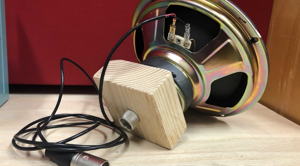
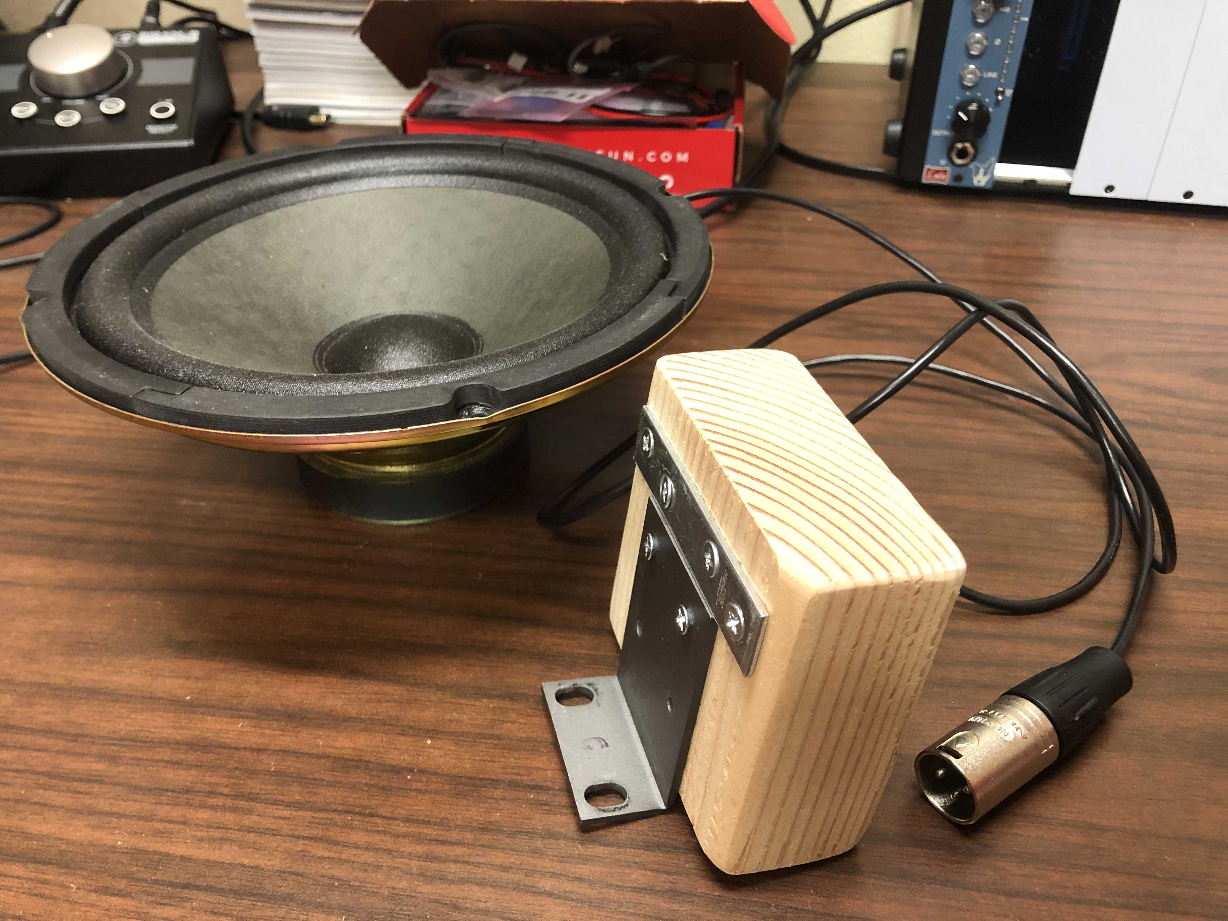
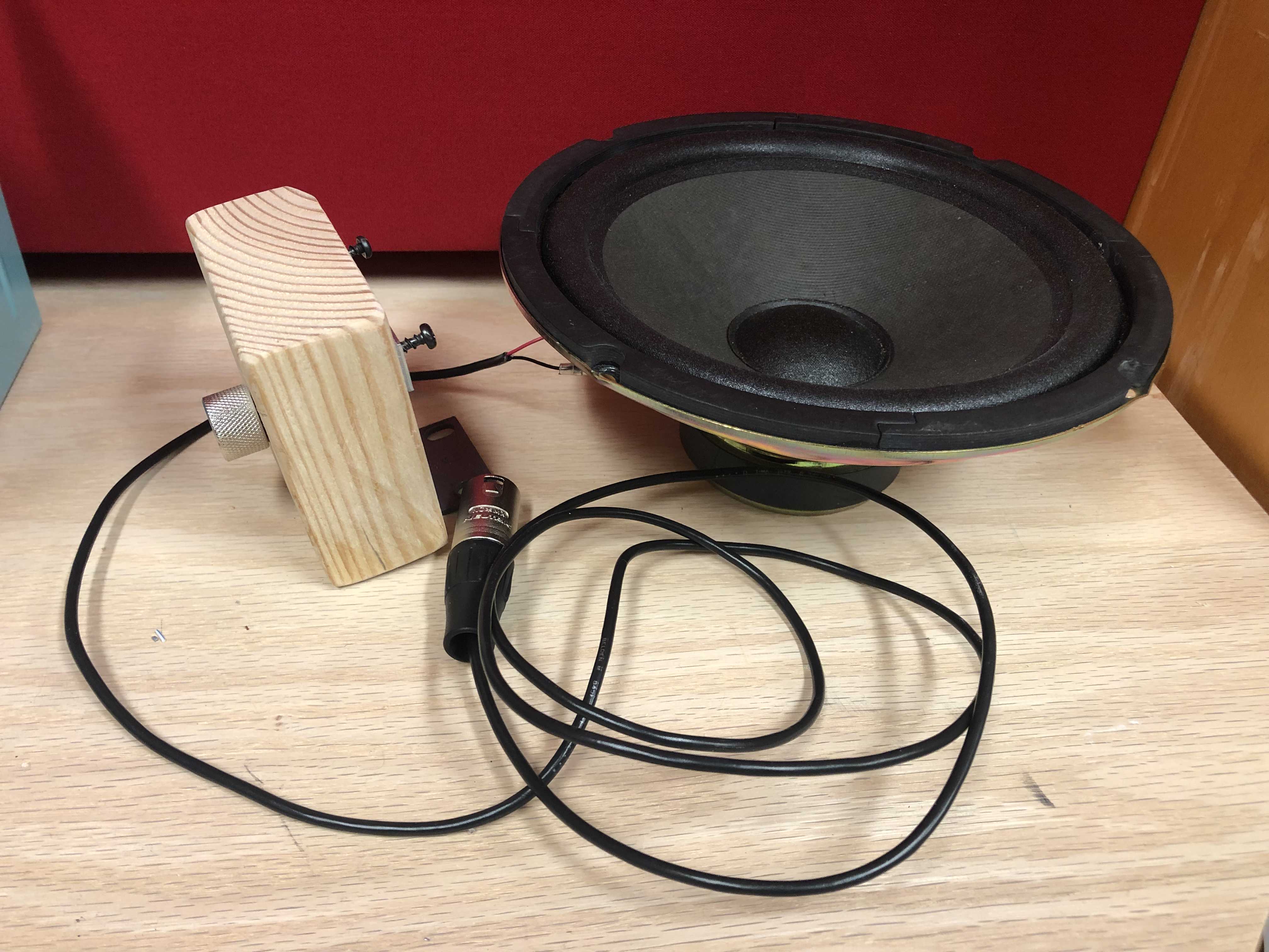
I had some leftover parts and speakers from sound art projects, so I decided to make a sub-kick mic.
I used a 6.5″ driver, a XLR Male end, a few feet of audio cable, and I custom build a mic clip for the mic using a 3/8″ to 5/8″ mic screw adapter, scrap wood, and some scrap metal.
Solder the XLR pin 2 to positive terminal (+) and pin 3 to the negative terminal (-). Cut off the ground (other posts state one could solder this to the speaker). I used spade speaker connectors so I could reuse the speaker for another project if I needed to.
For the stand, I had old rack ears that I screwed into a 2×4 that the magnet of the speaker clings to and the simple ledge helps brace the speaker. For the mic clip, I screwed in a 3/8″ to 5/8″ mic screw adapter. If necessary, one can add screws to further assist the magnetic hold onto the clip (see image below).
That’s it! No need to add a -20dB pad. You can use line input if necessary or pad it up on the mic preamp. I tested using my DIY Lola Mic Pre from Hairball Audio. Audio recordings are forthcoming…
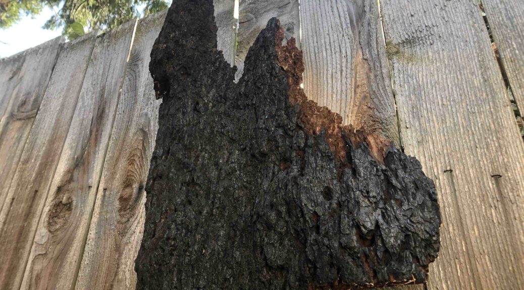
Over the summer, I produced five sound sculptures centered around fire-affected areas of the 2020 Holiday Farm fire. The work was part of the Soundscapes of Socioecological Succession (SSS) project that was funded through a Center for Environmental Futures, Andrew W. Mellon 2021 Summer Faculty Research Award from the University of Oregon.
Through field recording fieldwork, local wood sourcing, and custom electronic design, the five (5) sound sculpture prototypes were one way to generate a unique auditory experience aimed at the general public. The work was designed to unpack the sounds and scenes of wildfires in natural and human-systems and to document the regenerative succession of coupled social and ecological processes.
Video 1. Sound sculpture C prototype. Burnt cedar wood and audio sourced from fire affected area near Blue River, OR.
Socioecological systems emerge from interdependent processes through which people and nature self-organize across space and time (Gunderson and Holling, 2002). STEM-centric studies of socioecological dynamics miss literal and metaphorical connections between people and nature, which are difficult to quantify and to communicate. To address this limitation, the sound sculptures test a new approach to capture SSS as a qualitative record of collective response to catastrophic wildfire.
Like a slice of tree ring that marks age and time, the field recordings of audio in visits to fire-affected areas connotes a slice of succession activities. Sound recordings of the area are meant to capture multiple scenes and ecological voices, filtered through a raw material from the sites themselves.
Video 2. Sound sculpture D prototype. Wood and audio sourced from fire affected area near Blue River, OR.
Our sonic environment is polluted by man both in its content and its reflections. This is certainly true even for field recordists who venture further and further into the wild to break free from the noise pollution of a passing airplane, a highway’s din, or even audible underground activity such as fracking (One Square Inch, 2021). Treating site-specific wood as an acoustic resonator — a filter that distorts as much as it renders sound audible — casts a shadow onto the sounds it projects. The physical material acts as a filter upon the sound. The wood slightly changes the spectrum of sound by boosting or cutting the amount of different frequencies in the sound.
Our University of Oregon team expanded previous research by sampling the rich SSS at fire-affected sites, including soundscape field recordings, recorded interviews, and collecting “hazard tree” waste material. These materials offer a document of the resiliency of the landscape and illustrate how forest disturbance can set back human-defined sustainable development goals regionally. The development of the five sound sculptures are just one means to inform the public and inspire collective action towards sustainable futures.
Video 3. Sound sculpture E prototype. Wood and audio sourced from fire-affected area near Blue River, OR.
Audio field recordings were captured during two site visits to fire-affected areas on June 16, 2021 and July 2, 2021. The second visit was to H.J. Andrews forest and an interview and tour with Mark Schulze (H.J. Andrews Experimental Forest Director) Bailey Hilgren and I used a few field recording setups, and which mostly consisted of Bailey recording with a Zoom H6 using on-board mics and I recording with a Sound Devices 633 field mixer and three mics: Sennheiser MKH 30-P48 and MKH 50-P48 microphone in mid-side configuration and a LOM Uši Pro omnidirectional microphone. The Zoom recordings were captured at 96k-24bit, and the 633 recordings were captured at 192k-24bit. During the second visit, we were able to setup “tree ears” that consisted of two Uši Pro mics taped to a tree and a LOM Geofón low frequency microphone, and which we left recording for several hours in the H.J. Andrews forest (see Figure 2). Bailey organized all the audio recordings using the Universal Category System (UCS). The system is a public domain initiative for the classification of sound effects. While we chose not to make the 30+GB of audio files as a publicly available archive, we have made the audio categorization spreadsheet publicly available (SSS metadata spreadsheet).
Figure 1. Field recording setup at fire affected site.
Figure 2. “Tree ear” field recording configuration.
During the technical design phase, some secondary research questions were asked. Which audio exciter/transducers work best on non-flat, raw wood surfaces? Which exciters are the most cost-effective solution for an array of speakers?For fabrication of installing wood as pieces on a wall, can I cost-effectively source sturdier materials than aluminum posts?
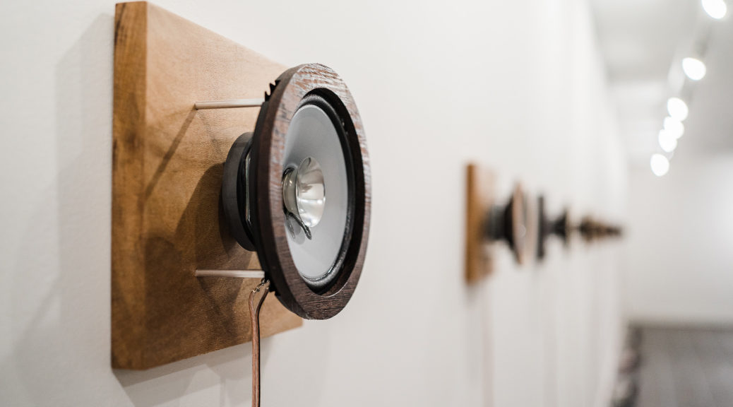
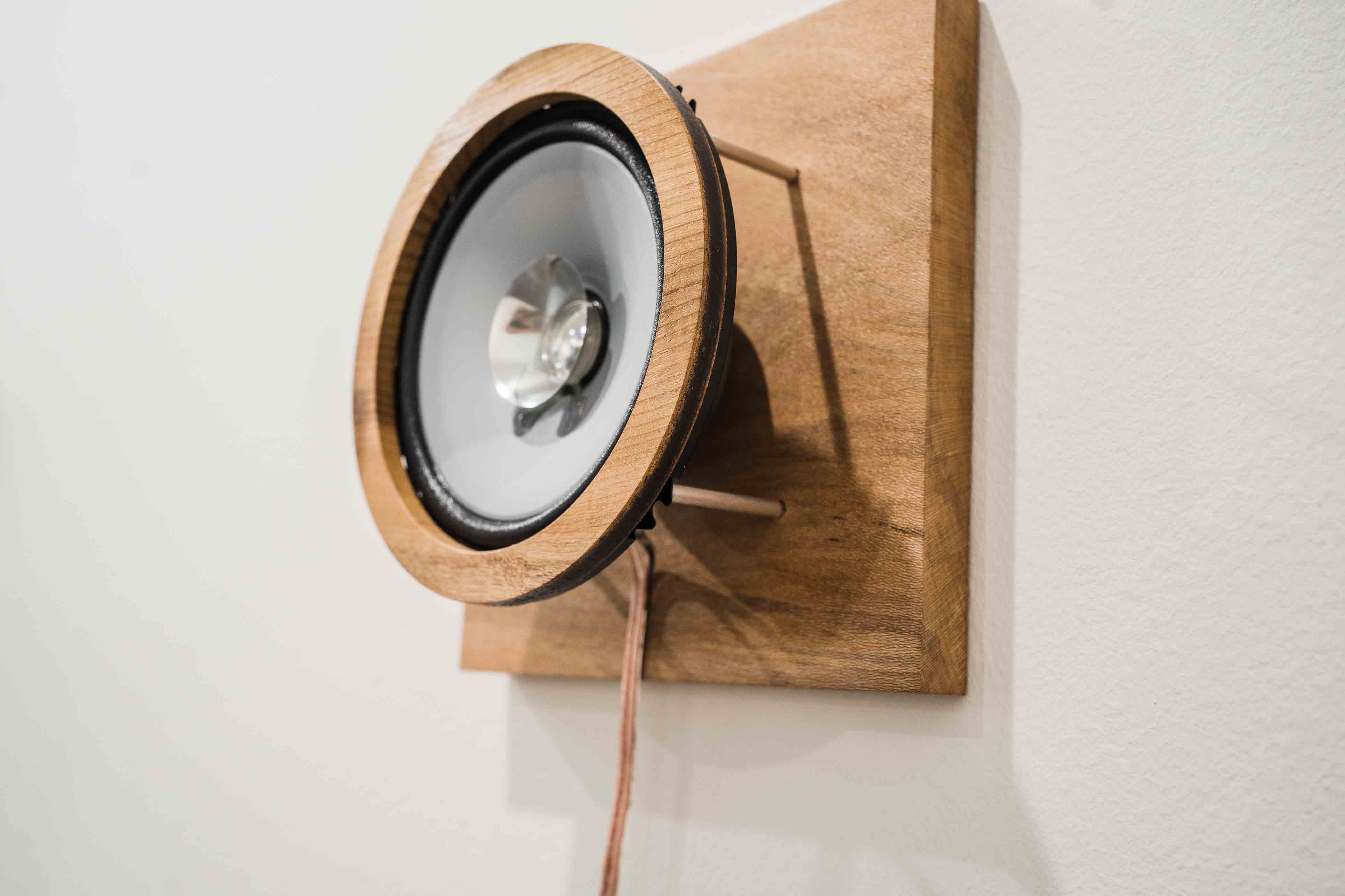
Figure 3. Sound sculpture prototypes depicting standoffs and speakers.
I tested a few different models: waterproof transducer, round and square exciters, and distributed mode loudspeakers. I also tested different speaker formats: 10W 8ohm, 20W 4ohm, and 20W 8ohm. Unfortunately, the desired power outputs, 25-30W, models of exciters were consistently sold out throughout the project, therefore I was unable to equally distribute testing across similar power outputs. From experience more than a scientific A/B test, I found that the more flexible options for attaching to wood surfaces were the Dayton Audio DAEX25Q-4 Quad Feet 25mm and the Dayton Audio DAEX32SQ-8 Square Frame 32mm Exciter, 10W 8 Ohm. Generally, I realized that in order to get decent output in both frequency response and gain, the low-end of $15-20/transducer seems about right. I do not recommend anything below 10W for this type of work. Getting a stereo image was not important and would be difficult given the size of wooden pieces. I valued volume and minimizing visual distraction, so speakers were meant to be placed behind or under the sculptures. I doubled speakers whenever I used 10W drivers.
Figure 4. Recording log loader moving hazard tree material
Audio 1. Log loader field recording (see Figure 4)
For standoffs, I sourced variable size stainless steel standoff screws used in mounting glass hardware which worked extremely well on the river wood sound sculpture (Figure 5).
Figure 5. Stainless steel standoffs, 10W 8ohm speakers, and custom electronics board on sound sculpture D prototype.
I sourced audio amplifiers on sale for under $10 each, where $15 is normal pricing. The TPA3116D2 2x50W Class D stereo amplifier boards have handled well on previous projects, and finding them cheaply with the added volume control and power switch were a great addition for fine-tuning amplification in public spaces.
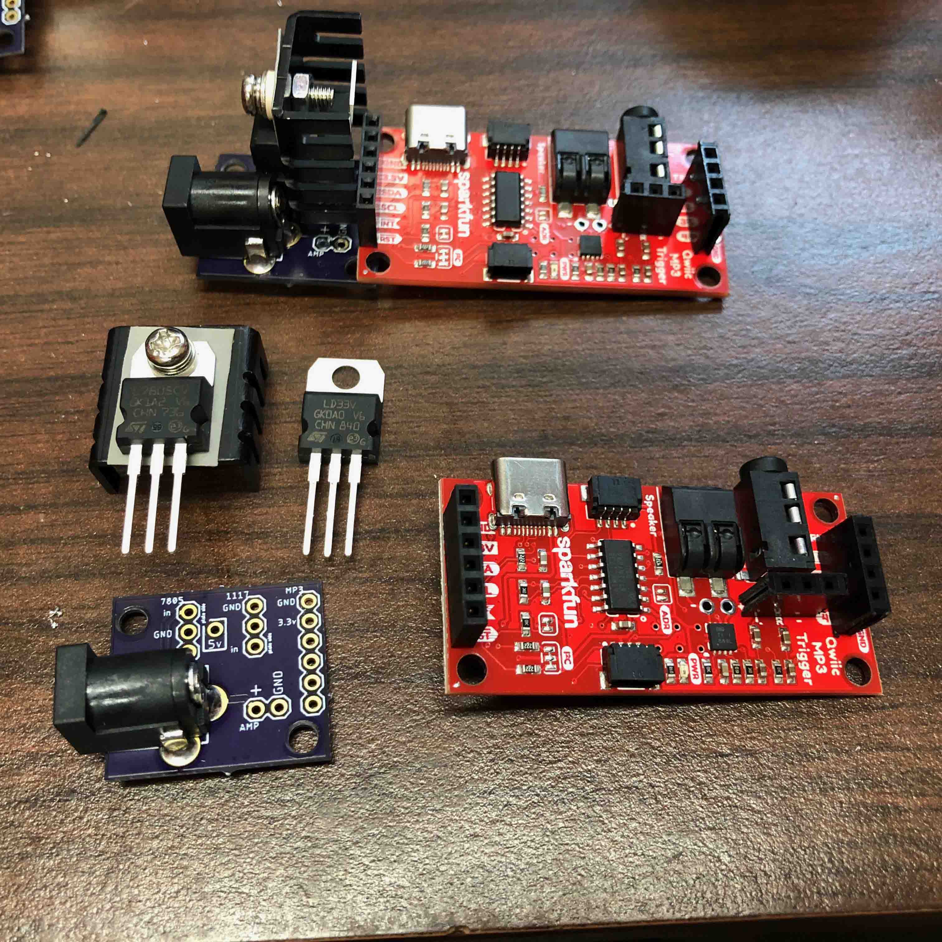
Normally powering the amplifiers and audio boards is where the real cost comes in, and I was happy to learn that Sparkfun’s Redbaord Arduino’s can now handle upwards of 15VDC, so I went with their MP3 Player Shield and Redboard UNO in order to split VDC power between the amplifier and board (12V, 2A power supplies were adequate for the project and transducer wattage).
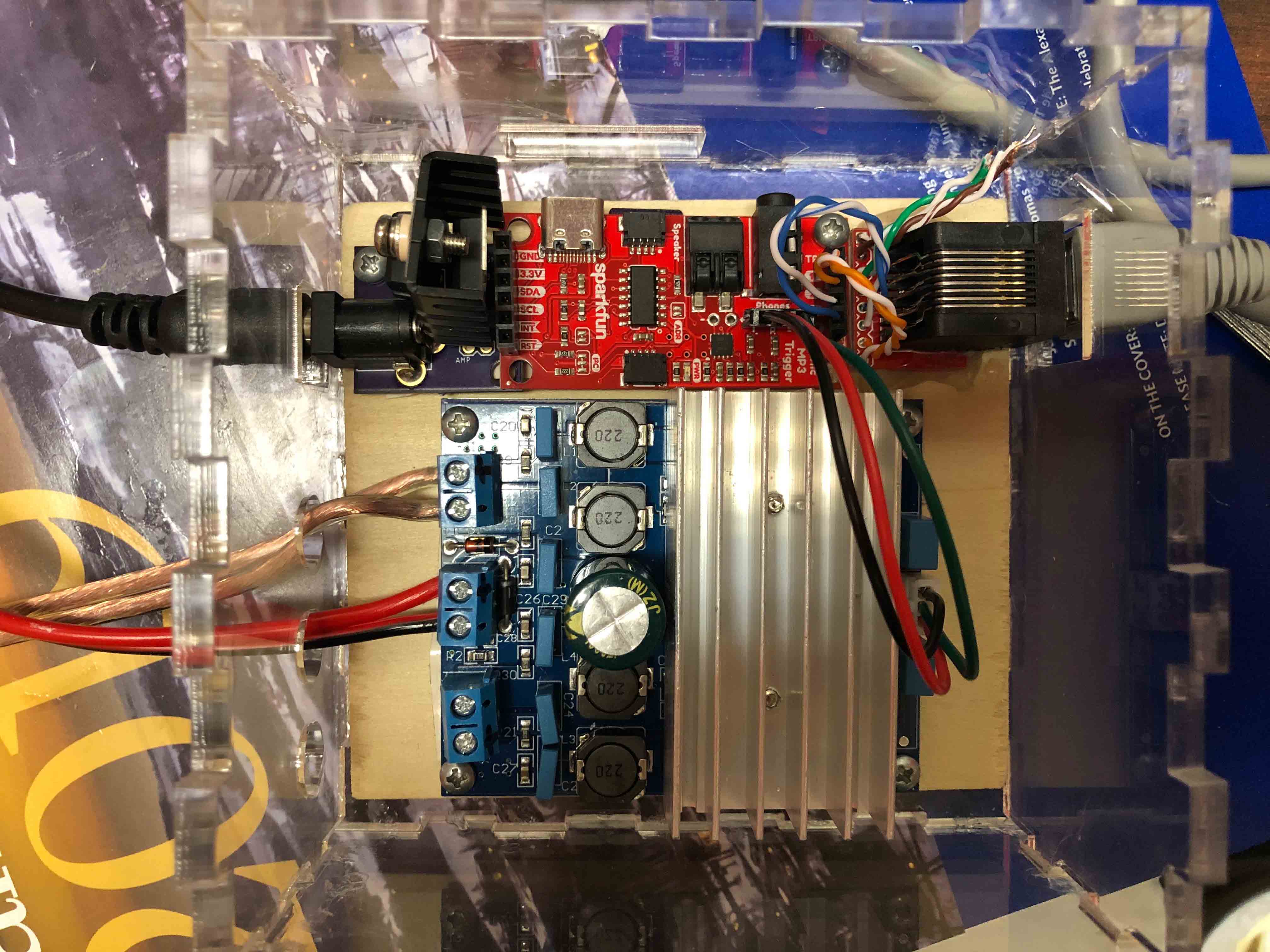
Figure 6. Custom electronics board consisting of MP3 player shield, Arduino UNO Redboard, 2x50W class D amplifier, and power split for up to 15VDC.
Figure 7. Recording site near Eagle Rock along the McKenzie River.
I modified the outdated MP3 player code on Arduino to dynamically handle any number of tracks and named audio files, such that one doesn’t need to rename audio files in the convention “track001.mp3” “track002.mp3”.Whatever audio files are uploaded onto the SD cards, the filenames simply need to be placed into an array at the top of the code uploaded to the board. Thus, when powered on, the sound sculpture will play an endless loop of the uploaded audio files found on the SD card.
***For those interested in the Arduino code running on the MP3 players, I have made the code publicly accessible as a repository on Github.
Figure 8. Full electronics module example: 12V 2A power supply, MP3 player shield, Sparkfun Redboard Arduino, TDA 2x50W stereo amplifier, single 10W exciter.
Video 4. Sound sculpture A prototype. Wood and audio sourced from fire-affected area near Blue River, OR.
Selecting the audio for sound sculptures came through discussions with Bailey around ecological succession, the interviews conducted, and the types of audio that was captured and categorized. We chose four audio bins (categories) to work with: animals, soundscape or ambient, logging or construction, and scientific or interviews. Again, Bailey created a categorical spreadsheet of audio files within these four bins.
Video 5. Sound sculpture A prototype. Wood and audio sourced from fire-affected area near Blue River, OR.
Constructing the sound sculptures involved imagining public space and the materials. There are two pieces for wall, one for hanging, one for a pedestal, and one for the ground. The sculptures are stand alone pieces that simply require AC power for showing. See below for a gallery of stills of these works.
CONCLUSION
By activating sourced raw materials (e.g., “hazard tree” wood) with acoustic signals stemming from local sites, the sound sculptures amplify the regional and collective voice of wildfire succession even as it outputs a modified version of the input sound.
The process of developing sound sculptures led to additional ideas for iteration or for incorporating the sculptures within a larger-scale project. For example, in our interviews with Ines Moran and Mark Schulze, we found out about “acoustic loggers,” battery operated, weather-proof audio field recorders that record audio based upon a timer. We ordered one such acoustic logger for the project, an Audio Moth; however, the Audio Moth order did not arrive after the completion of the project. Working these into the project through sampling fire-affected sites would create a unique dataset.
The sound sculptures can be stand-alone works. We appreciated the modular approach to the design, and we could continue the modular approach or tether sound objects together. Future work could involve spatializing audio across multiple sculptures similar to previous sound artwork, like Wildfire and Awash.
For the sound sculptures themselves, there is gain control on speaker-level but not on the line output of the players. We could add buttons for increasing/decreasing volume on the MP3 boards to better manage levels, and if we want to provide an interactive component to the works, we could buttons for cycling through tracks on sound sculptures.
Listening to our environment is essential. In 2015, The United Nations Educational, Scientific, and Cultural Organization (UNESCO) formed a “Charter for Sound” to emphasize sound as a critical signifier in environmental health (LeMuet, 2017). By continuing to incorporate sonic practices (bioacoustics, sound art, field recording) into our work with the environment, we create more pathways to experiencing and understanding the planet we live on.
References / Resources
Gunderson, L.H., Holling, C.S., 2002. Panarchy: Understanding Transformations in Human and Natural Systems, Panarchy understanding transformations in human and natural systems. Island Press. https://doi.org/10.1016/j.ecolecon.2004.01.010
The sound sculptures were made possible through a 2021 Center for Environmental Futures Andrew W. Mellon Summer Faculty Research Award in collaboration with Lucas Silva (ENVS).
A shout out to Thomas Rex Beverly from whom I got the idea about recording using the “tree ears” configuration.
This is a short article on creating video spectrograms (time-frequency plots) of audio files. The work comes from research project, Soundscapes of Socioecological Succession, funded by a Center for Environmental Futures, Andrew W. Mellon 2021 Summer Faculty Research Award.
The example in Video 1 is a spectrogram video created using Matlab. The audio is a recording of a small dynamite blast of a 70″ stump across from Eagle Rock, just past Eagle Rock Lodge on the McKenzie Hwy in Vida, OR.
Video 1. Video of spectrogram with playback barline and synchronized audio file.
I love spectrograms. I’ve worked with time-frequency plots in various ways in the past, namely spectral smoothing music (listen on Spotify), collaborative research (read the paper), and even teaching (Data Sonification course) at the University of Oregon. Yet, I am still amazed by the work of spectrograms and sound in the sciences. I knew of the theories around animals occupying various frequency spaces within a habitat based upon the bioacoustics work of Garth Paine and great multimedia reporting by Andreas von Bubnoff. Yet, after an interview with a UO visiting researcher, Ines Moran, as part of our Soundscapes of Socioecological Succession project, I was further intrigued by how sound, spectrograms, and AI plays an integral role in her bioacoustics research on bird communication.
This led me to revisit my work with spectrograms. I was blown away by Merlin ID’s auto spectrogram video app, and I wanted to relook at how I create my own spectrogram videos. I’ve been frustrated with multiple software solutions to generating scrolling spectrogram videos. Not having a seamless solution other than using screen capture on iZotope RX or Audacity spectrograms, I did some more research looking at iAnalyse 5 software (replaces eAnalysis software) and Cornell Lab’s RavenLite software, but was unsatisfied with movie export results. I appreciated the zoom functionality of each software but wanted auto-chunking or scrolling of the spectrogram within a high-resolution video.
I didn’t easily discover a straightforward plug n’ play solution (although I’m open to hearing one if you have a suggestion!). I ended up going back to Matlab to see if I could find a pre-existing library or code I could implement. I found slightly different versions, and not exactly seamless. I ended up refashioning some pre-existing code written by Theodoros Giannakopoulos that generated gifs from spectrograms. See gif Figure 1.
Figure 1. Original Gif export using pre-existing Matlab code.
I used this code as a starter for me to build out the function to export videos of spectrograms, and which I can specify the length in seconds for each window. Video 2 depicts example display output of audio waveform and the spectrogram of a Swainson’s Thrush bird call. I sync’ed the audio afterward in Adobe Premiere. I removed the waveform to focus on the spectrogram, and I had to get fancy on x-axis labels to dynamically match the length of windows that could be any length of seconds.
Video 2. Video output on a single screen, with split waveform and spectrogram view.
While I was unable to get a scrolling spectrogram video in one software, the auto-chunking feature was quite time-saving. I simply crafted an Adobe Premiere template with a scrolling animation graphic that I can easily edit to equal the exact window length and sync my original audio file to the movie. All within about a minute or two (see Figure 2). The final version has a nice scrolling playback bar on pages of spectrogram videos.
Figure 2. Screenshot of Adobe Premiere with line graphic that keyframe animates across the spectrogram during playback.
Video 3 displays the spectrogram complete with audio waveform, audio file, and playback barline (audio and playback barline added in Adobe Premiere).
Video 3. Video example with scrolling playback barline
Video 4 shows the final version of the code output after removing the audio waveform, resizing the graph, and updating the title. Again, adding the playback barline and synchronizing the audio were done in Adobe Premiere.
Video 4. Final version of Matlab code that generates a 1920x1080p spectrogram video the same length as the audio file.
The code gave me an easy way to label the spectrogram and embed this in the video. There are four steps.
1. Run the script in Matlab which outputs the 1920×1080 video and contains the same length as the audio file,
2. Drag the video into Adobe Premiere with the Graphics playback bar template
3. Drag the audio into the start to match the animation
4. Export the 1920×1080 video.
The process for one audio file takes about 2-3 minutes from start to finish.
I could make this more dynamic by grabbing the audio file length automatically and setting the frame rate automatically to match. simply determine how many “screen/pages” I want by editing the function variables.
***For those interested in the Matlab code, I have made it publicly accessible as a repository on Github.
Inspiration for the work was after an interview with Ines G. Moran, visiting scholar at the University of Oregon, who works in wildlife bioacoustics (website).
Are streaming services ready for dynamic random-order concept albums?
Random Playback is a music album that explores using dynamically looped playback to generate a unique listening experience for your own device (and which never ends). The album leverages streaming technology to randomly playback material endlessly and aims to simultaneously test the boundaries of streaming services’ “gapless playback“ feature. Just hit shuffle, repeat, and play.*
The Random Playback album consists of twelve loopable tracks of equal length that have no audio fades. The source material was generated and recorded with permission from playing an iOS clicker game, Rhythmcremental, created by Batta (Simon Hutchinson and Paul Turowski). In the game, sonically one advances by adding different instruments and triggers, thereby creating more rhythmic density and harmonies. Do check out the game. It’s addictive.
The tracks on the album are sequenced sequentially, such that one could play the album straight as if listening back to a selection of a single game of Rhythmcremental. Yet, by turning “shuffle” mode on, and turning on “repeat,” the album will loop endlessly, navigating seamlessly** between random tracks on the album in order to weave together a listening experience unique to your device. But don’t take my word for it. Hit Shuffle, Repeat, and Play and check it out for yourself…. (recommend playback in the app!)
*phone apps for Amazon Music and Apple services are the most seamless for shuffle playback.
UPDATE 9/21/21: While Spotify is seamless on chronological, non-shuffle playback, Spotify seems to falter if randomizing playback (confirmed by other users). Amazon Music Unlimited, however, seems to handle randomization playback well, nearly seamless (from the phone app). Apple Music also has seamless shuffle playback from the phone app. That said, any browser playback has terrible audio drops between songs on shuffle mode for all services.
**”Seamless” is part of the ‘testing the boundaries of streaming technology’ bit. The track-to-track gapless playback result relies quite a bit on server bandwidth and the “Gapless Playback” feature of the one’s streaming service. At the time of writing this, sequential playback sounds more seamless than random “gapless” playback (on Spotify). Although, this could be my own device and data bandwidth.
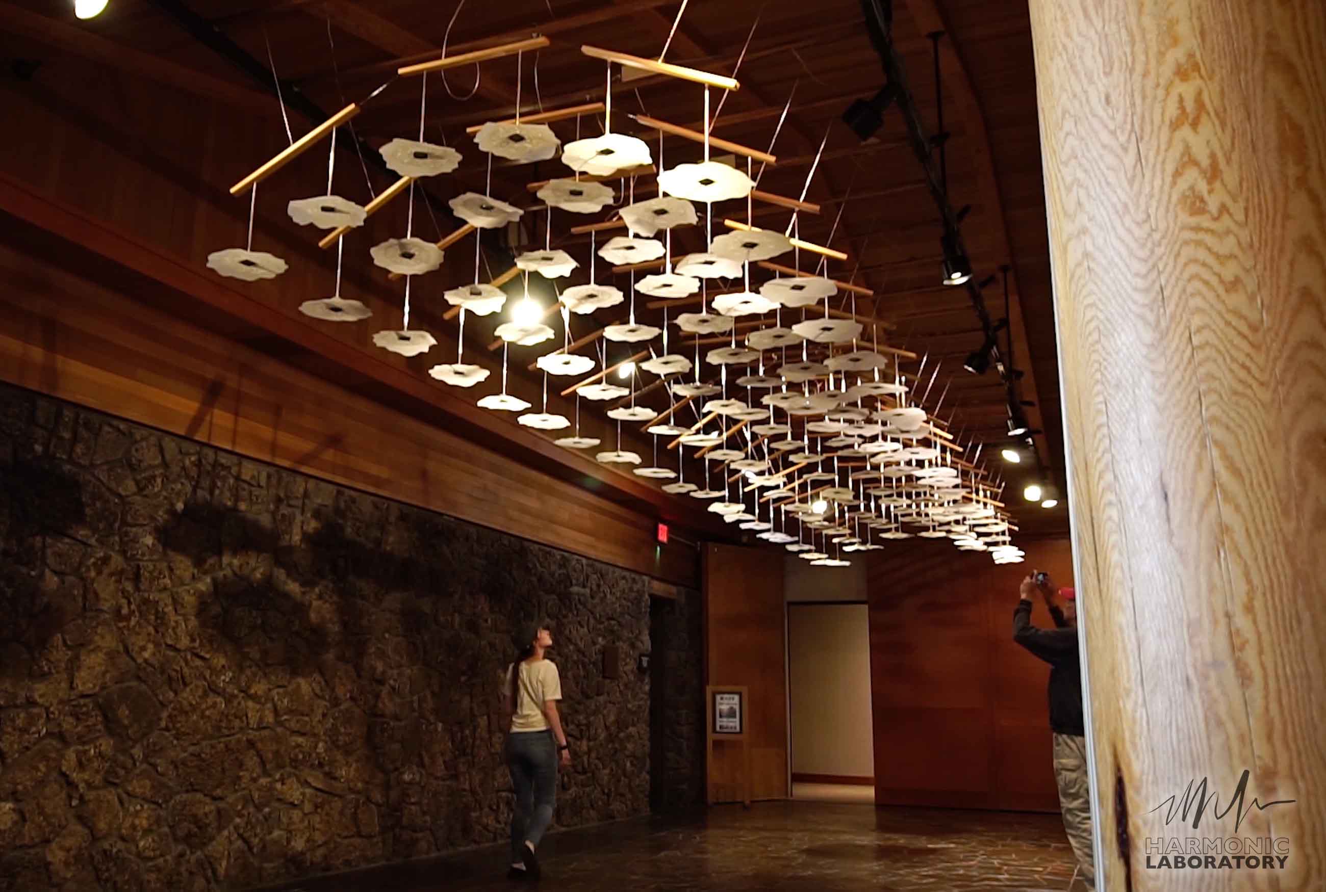
Wildfire is a 48-foot long speaker array that plays back a wave of fire sounds across its 48-foot span at speeds of actual wildfires. The sound art installation strives to have viewers embody the devastating spread of wildfires through an auditory experience.
Wildfire employs sound to investigate how the climate enables destructive wildfires that lead to statewide emergencies. The speed at which fires move can be mimicked in sound. By placing speakers along a surface (every three feet across 48 feet ~16 speakers), Wildfire implements spatialization techniques to play waves of fire sounds at speeds of simulated models and actual wildfire events. Comparing the speed of different fires through sound spatialization, we can hear how quickly different fires move across various wildfire behavior (fuel, topography, and weather).
Stereo audio example. Fire sound moving across stereophonic field at 16 mph.
Stereo audio example. Fire sound moving across stereophonic field at 83 mph.
Wildfire is comprised of sixteen 30W speakers, 120’ speaker cable, sixteen 8” square wood mounts, sixteen 6.25” diameter wood speaker rings, 64 aluminum speaker post mounts, eight custom electronic boards and enclosures, eight 50W power amps, one custom motherboard and enclosure, eight custom length Ethernet cables, custom-built power supply cable, sixteen 15V 4A power supplies, and three 9V 5A power supplies.
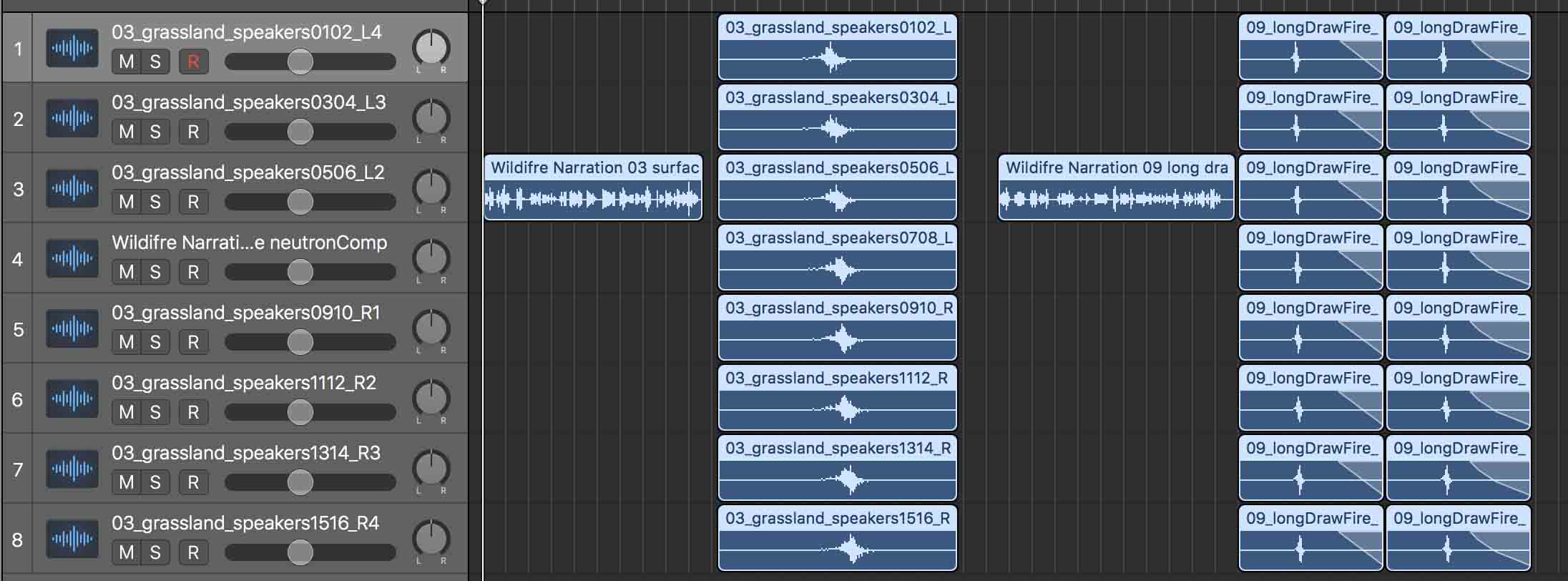
Eight different recordings of wildfire sound simulations are played across the 48-foot speaker array in looped playback. A narrator describes each wildfire event before the audio playback of fire sounds. Because audio on all eight stereo channels are triggered at the same time for simultaneous playback, audio spatialization is ‘baked-in’ on the audio files. The fire soundscapes are audio samples that have been simulated in a virtual space to move at speeds of actual wildfires and captured (read recorded) as eight stereo audio files at the same spatial location of the sixteen speakers in the physical world. The virtual mapping and recording process ensures little destructive interference as a result of phase shifts and time delays. I then mixed the resulting files inside Logic Pro X (see Figure below).
FIgure. Eight stereo audio files — each track represents audio for one sound FX board, which has stereo playback.
I am always amazed by how different topics are defined and vocabulary used when working across disciplines. For example, in seeking to play audio at varying rates of ‘speed,’ wildfire scientists and firefighters instead describe fires in terms of ‘rate of spread.’ Because fires are not single moving points but instead lines that can span miles moving in various directions all at once, speed is difficult for the field to put into practice. The term ‘spread’ and how it’s calculated serve wildfire science well but required me to think about how to convey the destructive ‘rates of spread’ as a rate a general observer may perceive along a two-dimensional speaker array (speakers mounted along a wall).
In order to distill wildfire science down to essential components for a gallery sound installation, I spent a lot of time speaking with various wildfire scientists on the phone, emailing various fire labs, working on estimating wildfire behavior using Rothermel’s Spread Rate model,[1][2] and working between the measured distance of ‘chains’ and miles. I am not a fire scientist; I am indebted to the help I received but any incongruencies are my own. I compiled eight narratives that juxtapose ‘common’ rates depicted in simulated models with real wildfires that have occurred in US western states over the past ten years based upon fire behavior (fuel, topography, and weather). These narratives are outlined in Table 1 at the bottom.
Earlier in the year, I worked with Harmonic Laboratory, the art collective I co-direct, on a 120- speaker environmental sound work called Awash.[3] The work was commissioned for the High Desert Museum in Bend, Oregon as part of the Museum’s 2019 Desert Reflections: Water Shapes the West exhibit, which ran from April 26 to Sept. 27, 2019. The 32’ x 8’ work evokes the beauty of the high desert through field recordings, timbral composition, and kinetic movement (Figure below).
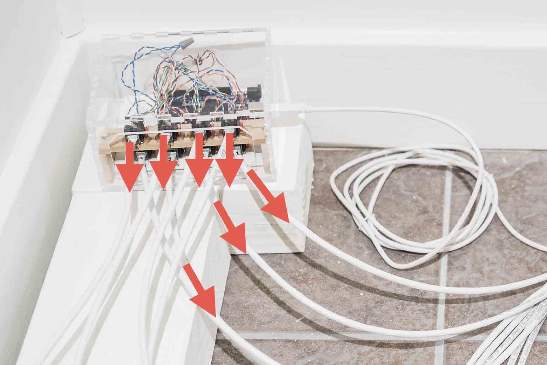
The electronic technology that I implemented in Awash for playing back audio across 120-speakers influenced my design of Wildfire. The electronics in Awash works by sending a basic low-voltage signal from the Arduino Mega motherboard to ten sound FX boards across Ethernet cable, thereby triggering simultaneous playback of audio across all 120-speakers (twelve 3W speakers per board powered by a 20W amplifier circuit). The electronics in Wildfire function in the same way: a low-voltage signal from the motherboard (Arduino Mega) is sent to eight electronic MP3 boards across Ethernet cable, thereby triggering simultaneous playback of audio across all sixteen speakers (Figures below). Instead of 3W speakers and 20W power amp boards used at the High Desert Museum, I chose to scale down the number of speakers and ramp up the wattage per board, choosing a stereo 50W power amp matched with two 30W speakers. The result is sixteen channels of audio running across eight stereo boards. And it doesn’t have to be sample-accurate!
Figure. Motherboard: Arduino Mega to eight Ethernet cable jacks.
Figure. Voltage trigger sent over Ethernet cable to each sound FX board. Any millisecond discrepancies in timing were inconsequential to possible phase interference due to the virtual audio recording process.
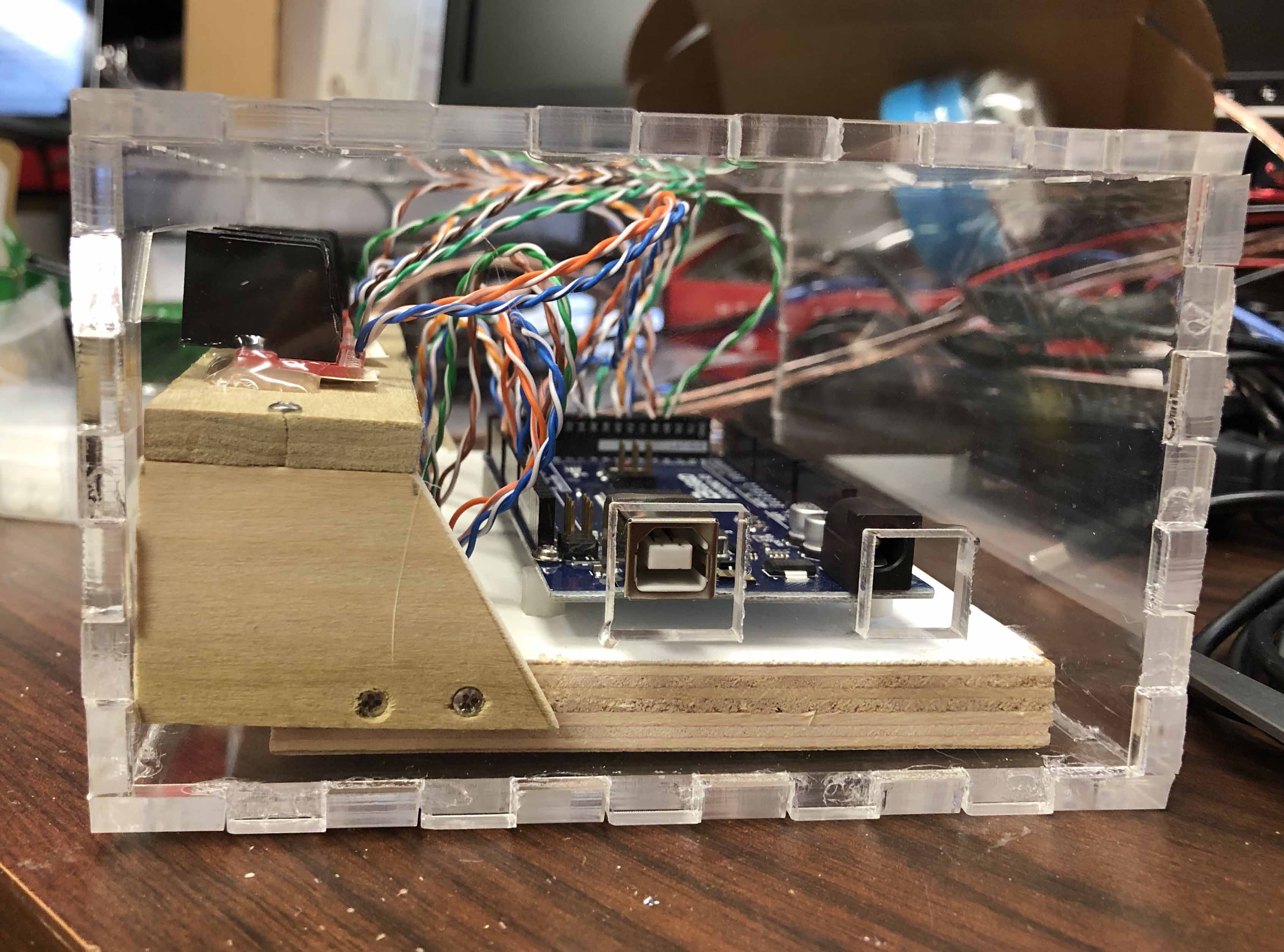
For Wildfire, I built custom laser-cut acrylic enclosures for the electronic boards (Figure below) using MakeABox.io (note: I found a good list of other services here). The second element was designing and creating custom PCB boards for the electronics themselves (Figure below). For the custom PCB board, I used Eagle CAD software (SparkFun has a great tutorial!) and then used an Oregon-based manufacturer OSH Park to print the boards.
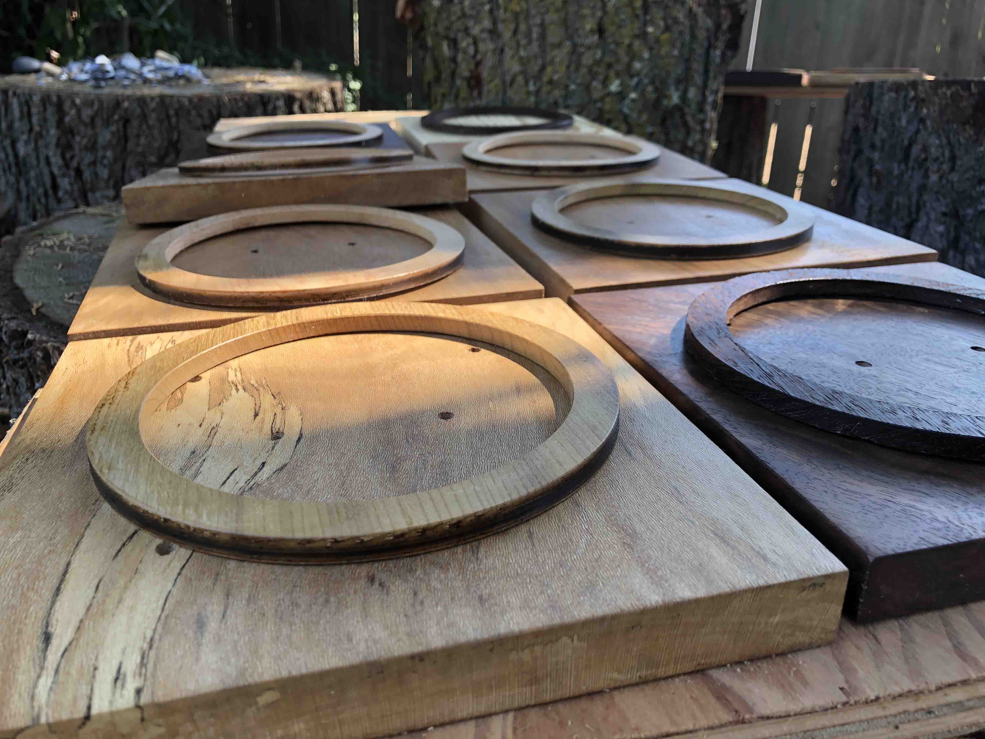
For the sixteen panel mounts and speaker rings, I sourced all wood from the woodshop at my father-in-law’s, who has various wood collected over the last 50-60 years. The panels were planed, cut, and drilled on-site and the speaker rings were cut using a drill press. The figure below depicts the raw materials after applying a basic wood varnish. The wood mounts consist of black walnut, pine, and sycamore woods. The wooden speaker rings consist of alder, ebony, and myrtle woods.
Figure. Six different woods used for speaker mounts and rings.
In the build-out, I was unable to power both the power amp and the MP3 audio boards from a single power source, even with voltage regulators. A large hum was evident during the split of power. A future work could attempt to power from a single power source while sharing ground with the motherboard. Yet, the audible hum led me to power the boards separately.
During install, I ran into issues of triggering related to the MP3 Qwiik trigger boards. The power draw for each MP3 board is between 3 to 3.3V, and I ran four boards from a single 9V 5A power supply using a custom T-tap connector cable and 1117 voltage regulators, in which I registered 3.26V along each power connection. However, upon sending a low-voltage trigger from the motherboard to the MP3 boards, I was unable to successfully trigger audio from the fourth and final board located at the end of the power supply connector cable. The problem remained consistent, even after switching modules, switching boards, testing Ethernet data cable, testing a different I2C communication protocol in the same configuration, among other troubleshooting tasks. When powering the final board with a different power supply (5V 2A supply), I was able to successfully trigger all eight electronic boards at once. It should be noted that the issue seems to have cascaded from my failure to effectively split power from a single power source per electronics module.
Figure. Electronics in Edith Langley Barrett Art Gallery, 2019. Photo by: http://janelleshootsphotos.com
The minimal aesthetic was slightly hindered due to the amount of data and power cables running along the floor. There is minimal noise induction with long speaker cable runs, such that in my second install at SPRING|BREAK in NYC, I relied on longer speaker cable runs instead of long power and data cables. Speaker cable is cheaper than power cable, so keeping costs down, saving time in dressing cables, and minimizing cabling along the 48’ span, focusing the attention on the speakers, wood, and audio. And, if I use the MP3 boards again, I would implement the I2C protocol and consolidate the electronics, which would save on data cabling.
Figure. Wildfire at SPRING|BREAK in NYC in March, 2020. Photo from SPRING|BREAK Instagram.
Through the active listening experience of hearing sounds of wildfires at realistic speeds, viewers are openly invited to support sustainable and resilient policies, including ones that can be done immediately, like creating defensible space around their homes. In the face of continued ongoing wildfires that become more frequent, Wildfire sonically strives to impact the listener in registering the devastation caused by wildfires. Getting the public to support sustainable policies and/or individually prepare for wildfires helps make communities more resilient to the impacts of wildfires and other disaster-related phenomena caused by climate change.
The work was made possible through the University of Oregon Center for Environmental Futures and the Andrew W. Mellon Foundation. The Impact! exhibition at the Barrett Art Gallery was supported with funds from the Oregon Arts Commission. Thank you to Meg Austin for inviting me to display work at the Barrett Art Gallery, and I am indebted to Sarisha Hoogheem and Matthew Klausner for their hard work in putting the show together. Thank you to Meg Austin and Ashlie Flood for curating Wildfire at SPRING|BREAK in NYC. And kudos again to Matthew Klausner and Jay Schnitt for their hard work in putting the piece up. Thank you to my cousin John Bellona, a career Nevada firefighter, for his insight on western wildfires and contacts in the field. Thank you to Dr. Mark Finney for providing common averages of speed-related to wildfires; Dr. Kara Yedinek for sharing insights on audio frequencies from her fire research; and Sherry Leis, Jennifer Crites, Janean Creighton and the other fire specialists who helped me along the way.
Table 1: Narratives in Wildfire
Feature
Characteristics
Rate of Spread
Time across 48-foot speaker array
Surface Fire: Grass
Yarnell Hill Fire, June 30, 2013
Crown fire: Forest
Delta Fire, near Shasta, California. September 5th, 2018
Surface Fire: Western Grassland, Short Grass
Long Draw Fire. Eastern Oregon. July 12, 2012
Crown Fire: Pine and Sagebrush
Camp Fire, near Paradise California. November 8th 2018.
Low dead fuel moisture content, High wind speed, Level terrain
Upper average forward rate of spread, 894 chains/hour
During Granite Mountain crew de- ployment, 1280 chains/hour
Upper average forward rate of spread, 297.6 chains/hour
Initial perimeter rate of spread, 16,993 sq. chains/hour
Perimeter rate of spread, 1250 chains/hour
Average perimeter rate of spread, 61,960 sq chains/hour
Perimeter rate of spread 525 chains/hour
Peak perimeter rate of spread, 67,000 sq. chains/hour
2.92 seconds
2.04 seconds
8.7 seconds
1.54 seconds
2.16 seconds
0.422 seconds
4.99 seconds
0.394 seconds
[1] F. A. Albini, “Estimating wildfire behavior and effects,” United States Department of Agriculture, Forest Service, Tech. Rep., 1976.
[2] J.H. Scott and R.E. Burgan, “Standard fire behavior fuel models: A comprehensive set for use with Rothermel’s surface fire spread model,” United States Department of Agriculture, Forest Service, Tech. Rep., June 2005.
[3] J. Bellona, J. Park, and J. Schropp, “Awash,” https://harmoniclab.org/portfolio/awash/
Sound art installations that require digital computing, especially projects that rely on advanced software, demand added insurance of stability in order to remain up in an unattended space for extended periods of time. For exhibitions, this time period can mean a month or more with hours that vary from business hours to a taxing 24-7. One added insurance for artists relying on computers (e.g., Mac Minis) for unattended digital works is the cron job.
A cron is “a time-based job scheduler” that runs periodically (time intervals) to help “maintain software environments” (footnote 1). A software utility for Unix (read Mac), the cron automates processes and tasks, allowing the computer to be used as your personal docent to check on installation software, updating variables as part of the work or fixing issues as they crop up.
I got into cron jobs in 2014 while I was working with John Park on #Carbonfeed (URL), a multimedia installation that leverages Twitter API to transform real-time tweets into physical bubbles in tubes of water as well as a musical composition driven by behavior on Twitter (Figure 1). The piece incorporates a custom node.js script running on a Mac mini. To anticipate power failures, and to even alter hashtag sets on the LCD screens (Figure 2), I needed a way to automate software processes and failsafes. Enter the cron job.
Figure 1. #Carbonfeed (photo by Janelle Rodriguez http://janelleshootsphotos.com)
Figure 2. #Carbonfeed hashtags (photo by Janelle Rodriguez http://janelleshootsphotos.com)
In #Carbonfeed, I used the cron to check if the software had crashed and automatically reboot, and every 8 minutes, I altered Twitter hashtag sets on the LCDs, in order to change the dynamic of the work and create new opportunities for discourse. For a how-to on the cron and cron specifics, please jump to the bottom of this article.
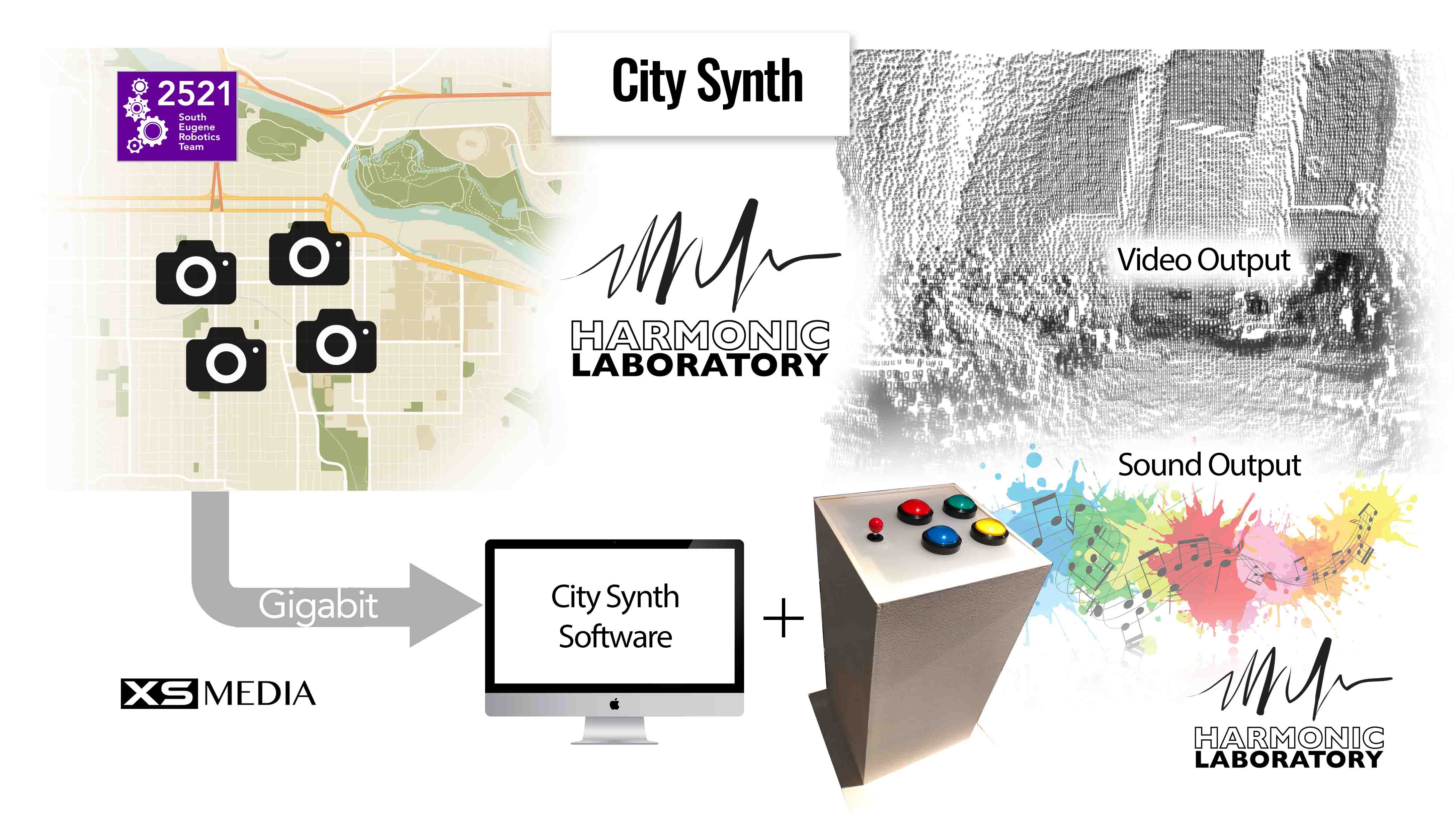
Since #Carbonfeed, whenever I found myself working on a sound installation that required advanced software (e.g., Processing, Max/MSP, Logic Pro X), I inevitably involved a cron. For example, in 2017, I worked with Harmonic Laboratory (URL) on a Mozilla Gigabit Foundation Grant (URL) project called City Synth, which turned the city of Eugene, OR into a musical instrument. The piece involved taking live video feeds from Raspberry Pis (a collaboration completed by the South Eugene Robotics Team, URL) that was mangled by a Processing sketch and subsequently controlled a live synthesizer running in Logic Pro X. The work was up for a month in the Broadway Commerce Center in downtown Eugene, OR.
Figure 3. City Synth signal flow diagram
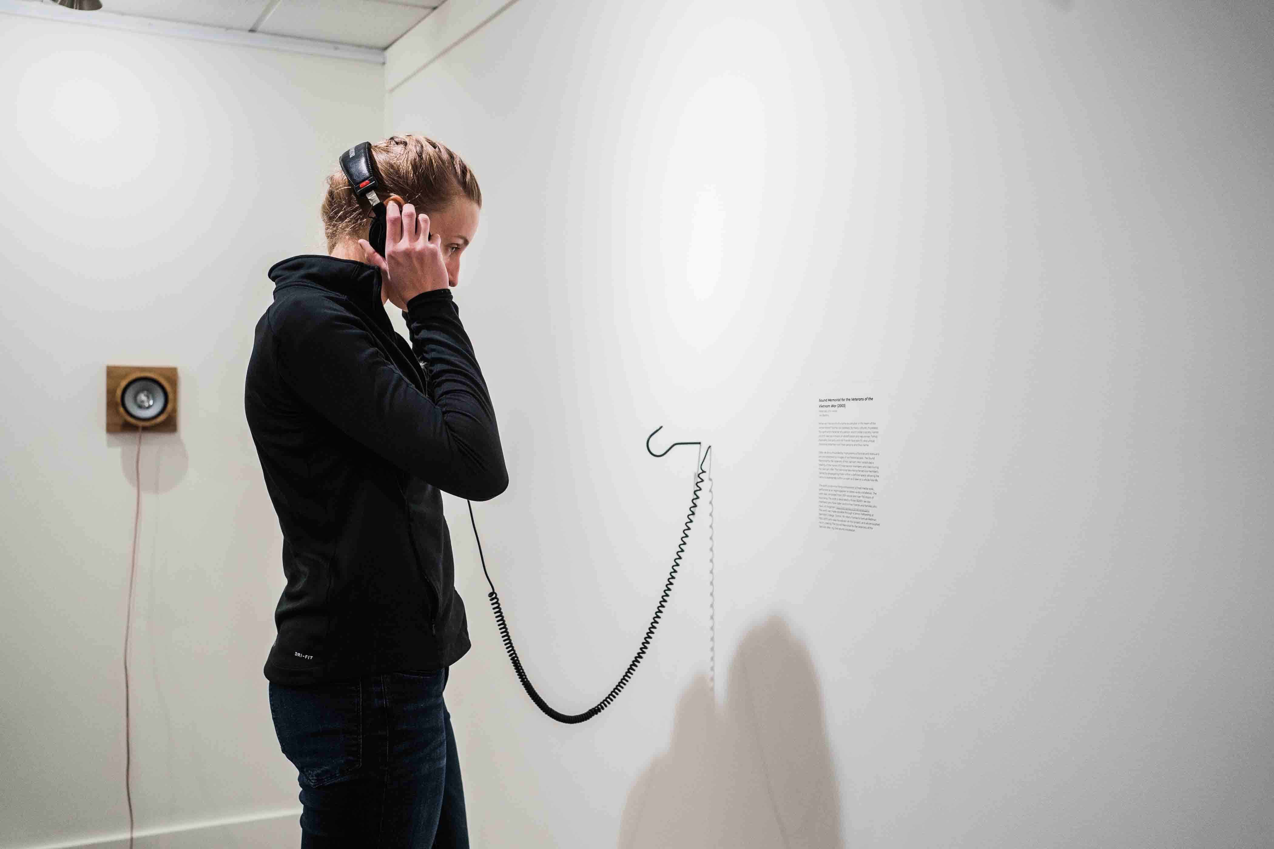
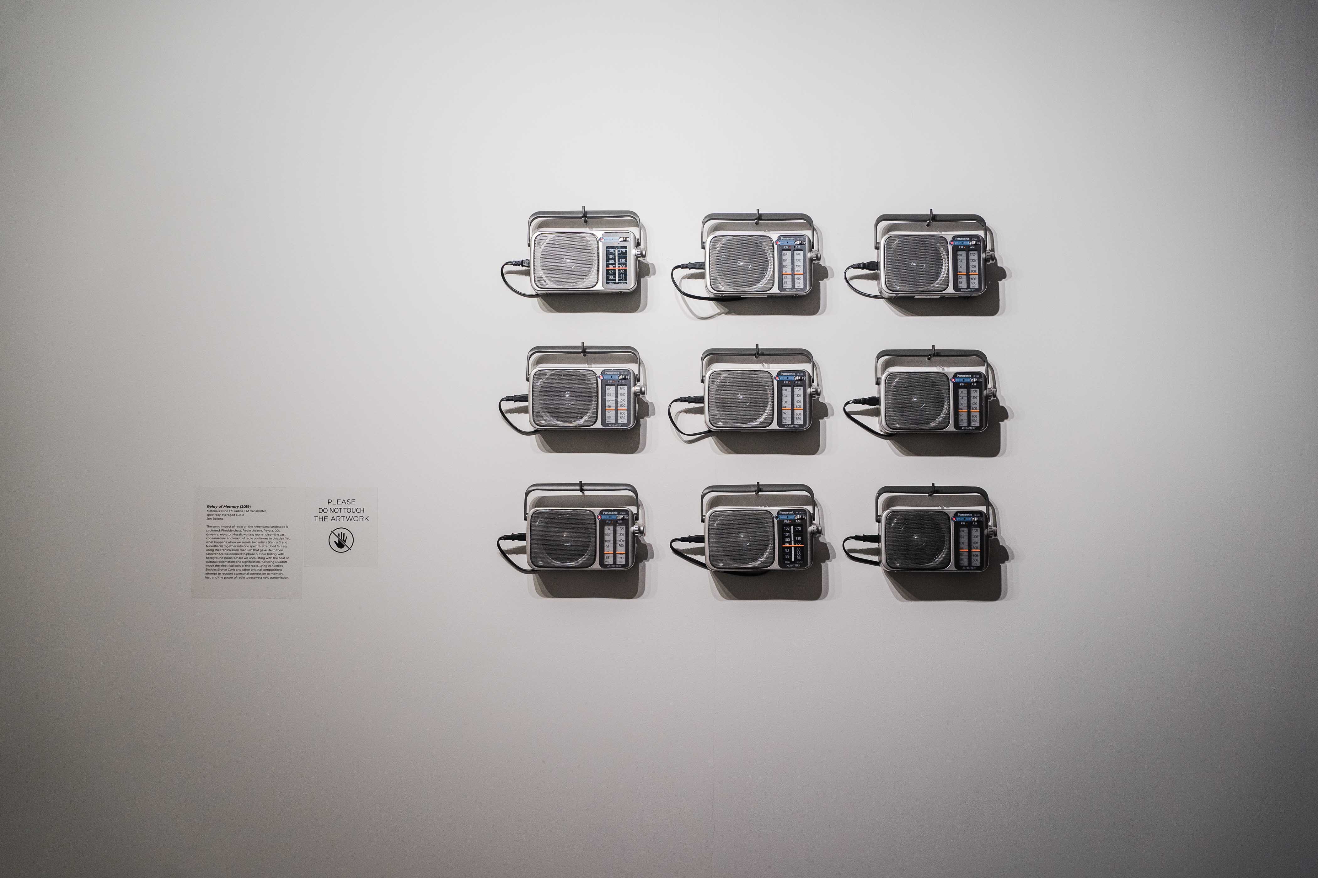
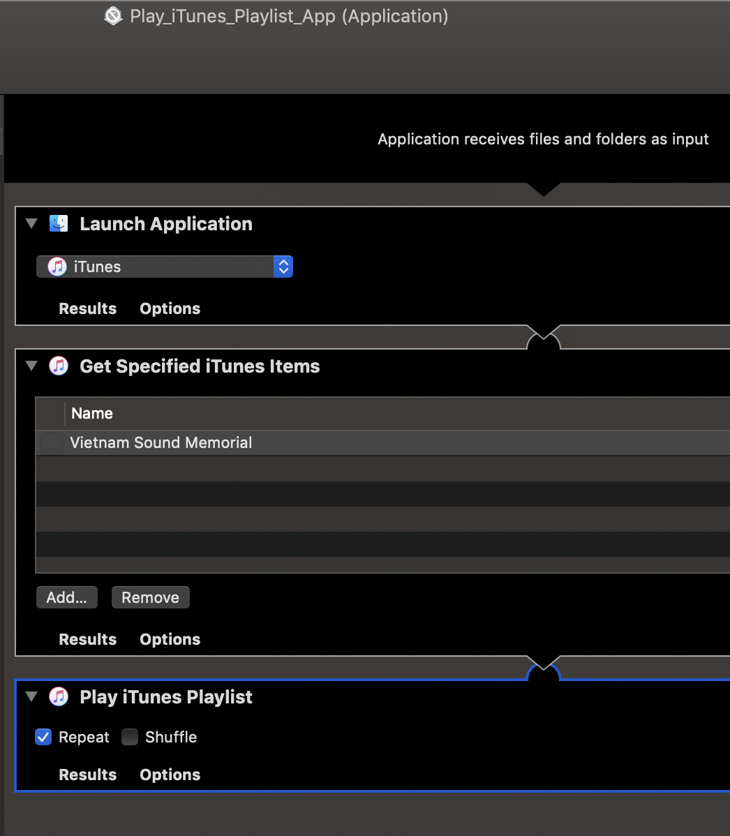
In 2019, my first solo exhibition at the Edith Barrett Gallery in Utica, NY (curated by Megan C. Austin and Sarisha Hogan and supported by funds from the Oregon Arts Commission) had six sound artworks running for three months. Since I was able to borrow Mac minis for the exhibition, I incorporated cron jobs and scripts to transform Mac minis into glorified audio players for two of the works. Sound Memorial for the Veteran of the Vietnam War (URL), ran an Automator script upon startup that opened iTunes and played a playlist holding the six-hour-long work (Figure 4). I mixed the 8-channel work down to a stereo headphone mix in order to account for the bleed of other works inside the space. Relay of Memory (URL) used the same script to output computer audio to an FM transmitter, which played the work through nine radios hung on a wall (Figure 5). Cron jobs checked the status of running software.
Figure 4. Sound Memorial for Veterans of the Vietnam War (photo by Janelle Rodriguez, http://janelleshootsphotos.com)
Figure 5. Relay of Memory (photo by Janelle Rodriguez, http://janelleshootsphotos.com)
The cron utility has been an amazing tool for my sound installation work. I can still recall driving home after installing Aqua•litative (URL) when I received a frantic call from the curator that there was a power outage. In the middle of the call, the power came back on, the computer turned on (setting to automatically start after power failure), and a minute later, the cron kicked in opening up all software. I didn’t need to turn around and drive back or walk the curator through how to turn on computer software. A happy moment.
I have saved countless hours that I know about, and I’m sure many other hours I won’t ever know about thanks to the cron. I even have started to implement the cron in other ways to help with basic tasks in my daily life (see below for code specifics) such that the cron has helped me get closer to what Allan Kaprow describes as the “fluid” and “indistinct” “line between art and life.” Maybe the overseer of digital automatons is what a 21st-century computing artist feels like (footnote 2).
CRON
This is a walkthrough of the crontab on Mac OS using Terminal. I’ve included some code specifics by theme below. If you use, please share your work with me and how you implemented your cron! If you like what you’ve read, sign up for my mailing list (URL), follow my music on Spotify (URL), and please share it with friends.
Setting up a cron
Googling helped me in every way possible for working with crontab, but there are three basic steps. Open up an editor via Terminal, add your cron code (requires setting a time of how often it’ll run), and then saving the file. For more on Terminal, here’s a beginner’s walkthrough, Apple’s user guide, and a command cheat sheet.
1. Open up an editor to add a cron via Terminal
env EDITOR=nano crontab -e
2. Inside the editor add the executable file to the cron job
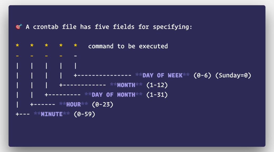
The asterisks tell how often to run the cron: Minute, Hour, Day of Month, Month, Day of Week. Straight asterisks mean “every” so this is a call to run the cron EVERY minute. The cron after the timer is a call to run a bash script called “citysynth_cron.sh”. The below cron runs every 5 minutes and closes the bash window in Terminal.
*/5 * * * * osascript -e 'tell application "Terminal" to close (every window whose name contains "bash")';
3. Save and exit the cron.
Ctrl-O, saves the file. Ctrl-X exits the file. You must save the temporary file after editing. When you are done with the cron and want to remove the cron job, follow step 1 to open, but then delete the lines (using Ctrl-K) and save the file. For reference, see http://www.maclife.com/article/columns/terminal_101_creating_cron_jobs
4. Want to know if you have a cron on your machine? List your crons in Terminal with
crontab -l
Adding a bash script.
If you decide to run a bash script via a cron, you’ll need to make the .sh file executable, that is, give the cron the ability to run the script. In Terminal, navigate to the folder where the .sh file lives and change its permissions with
chmod +x bashfile_name
where “bashfile_name” is the name of the .sh script (make sure to include .sh in the filename).
Below is an example of a .sh script that checks to see if an app is running and if not, reopens the app. I included the initial bash line of the file in the code.
#!/usr/bin/env bash

echo "cron job";

PROCESS=api_hashtags-polyphonic
number=$(ps aux | grep $PROCESS | grep -v grep | wc -l)

if [ $number -gt 0 ]
    then
        echo Running;
else
	echo "sound is Dead";
	# open music player application
	cd ~/Music/carbonfeed/work/sound/;
	sleep 2;
	open api_hashtags-polyphonic.app;
fi
Doing it all in one line of code
For recent projects, I opted to run code directly via the cron instead of relying on bash and AppleScripts. Below is code to start the Chrome web browser at a random time (to the second!) between 855-9p.
55 20 * * * perl -le 'sleep rand 300' && open -a 'Google Chrome'
Remember, the timing of the cron comes first:: Minute, Hour, Day of Month, Month, Day of Week. The cron is fired at 8:55pm, but has a random sleep time (between 0-300 seconds, read between your 8:55–9:00) and THEN opens the web browser.
Adding in an Apple Script
You can use your cron to trigger an Apple Script (.scpt file), just another way to execute commands on your Mac. Here’s an example of telling Safari to hit the spacebar (or could even be iTunes).
tell application "Safari"
	activate
end tell
delay 2
tell application "System Events"
	key code 49 -- space bar
end tell
Automator scripts (triggered by cron or system startup)
If cron and bash aren’t your thing, Apple has the Automator app that allows you to create automated processes straight from a GUI and then save out as an application (Figure 6). You can also easily trigger the app via a cron or by system startup by going to System Prefs > Users > Login Items. Login items can be set to run Automator scripts upon computer startup, and configuring the computer to power up automatically after power failure will help ensure a work stays running.
Figure 6. Automator Script to open iTunes and play a playlist on repeat.
Hope this was helpful. Please get in touch if you have questions or want to share your work with cron in art.
Footnotes
1. Wikipidea, “Cron”. URL: https://en.wikipedia.org/wiki/Cron accessed August 27, 2020.
2. Allan Kaprow. Essays on the Blurring Between Art and Life. University of California Press, Los Angeles. 1993. URL
The keywords in this question are distribute and streaming. Digital distribution is the delivery of your music to digital service providers like Spotify, Apple Music, Amazon Music, TIDAL, Napster, Google Play, Deezer, among many other streaming platforms.
Digital distribution companies (CD Baby, DistroKid, RouteNote, Mondotunes, ReverbNation, Landr, Awal, Fresh Tunes, Tunecore, Chorus Music, Symphonic, etc.) help get your music onto these digital service platforms. Without a digital distributor, the doors to these outlets are pretty much closed. That said, distribution companies do NOT own your music. They may take revenue from royalties, but you retain your rights. Distribution companies are also NOT stand-alone stores (i.e. BandCamp) although some offer this service (e.g., CD Baby).
This document is a walk-through going over the steps to digital distribution, from start to release. Over the course of the walk-through, we will create a track and then release that same track on a digital distribution service (all free). The goals of the walk-through are to:
Understand the basics of digital distribution
Take some of the fear out of releasing your music online
Prepare for future self-release work
The walk-through should take about an hour, depending on your familiarity with audio software and a relaxed mind when it comes to generating names/titles.
The various components of releasing music in this walk-through consist of
Create a track for release (we will create a pink noise track)
Generate all materials associated with the release
Register with a digital distribution service (free)
Distribute your work with the digital distribution service
Following any additional steps you can take (PRO registration, SoundExchange, claim artist profile, digital store setup)
Since the hardest part of the release process is the music creation (right?), let’s just get over this hurdle by creating a noise track right now in the next five minutes. Don’t worry, we will create a pink noise track (for relaxation and sleep) to help us skirt around personal aesthetics, notions of perfectionism, genre, and all things that take time and intentional decision-making. If you have a music track already, just skip this next section.
1. CREATE A PINK NOISE TRACK FOR RELEASE
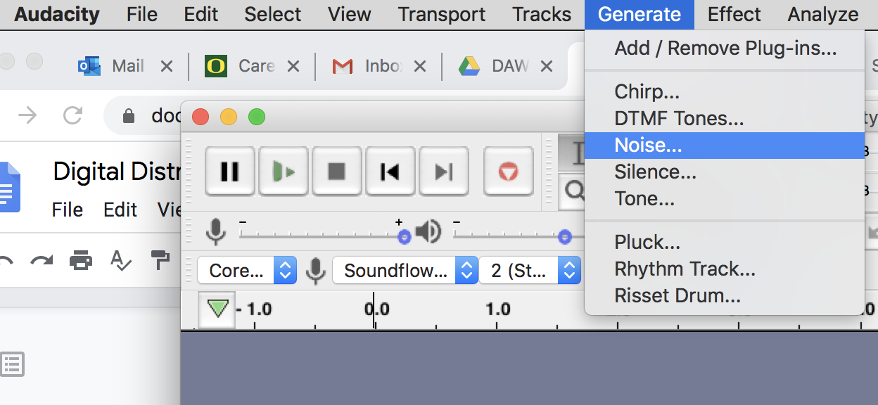
If you have a track for the release that you want to use INSTEAD of pink noise track(s), please skip this step. If not, read on. Open up Audacity (link) or any free software that can “generate” noise. Audacity is free and contains a noise generator.
Figure 1. Generate Noise menu in Audacity audio software
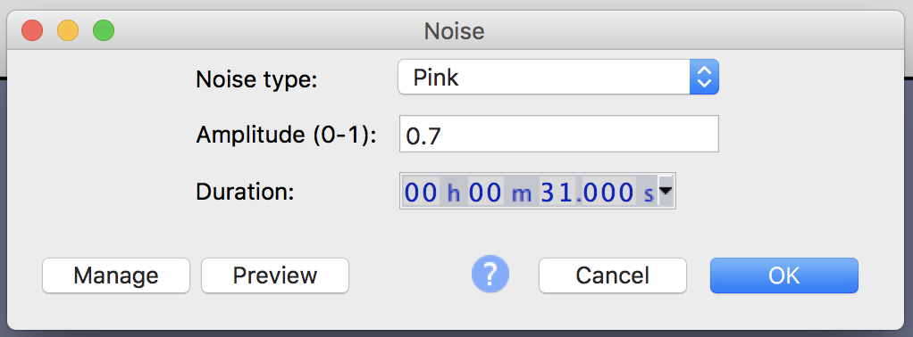
After selecting Generate > Noise… choose “Pink Noise” (of course you may choose White or Brown noise). Read about the differences here (link) (link). An amplitude of about 0.7 will work for pink noise as this will help keep the loudness units of the track in the correct range for streaming services. Read about LUFS here (link).
Choose the length to be between 30 and 40 seconds. We’ll want to choose the length to be ABOVE 30 seconds as streaming services (like Spotify and Amazon) only consider a “play” if thirty seconds of the track has been streamed. If you want your music to have “plays,” the tracks need to be longer than 30 seconds (footnote 1).
Figure 2. Noise generator settings in Audacity.
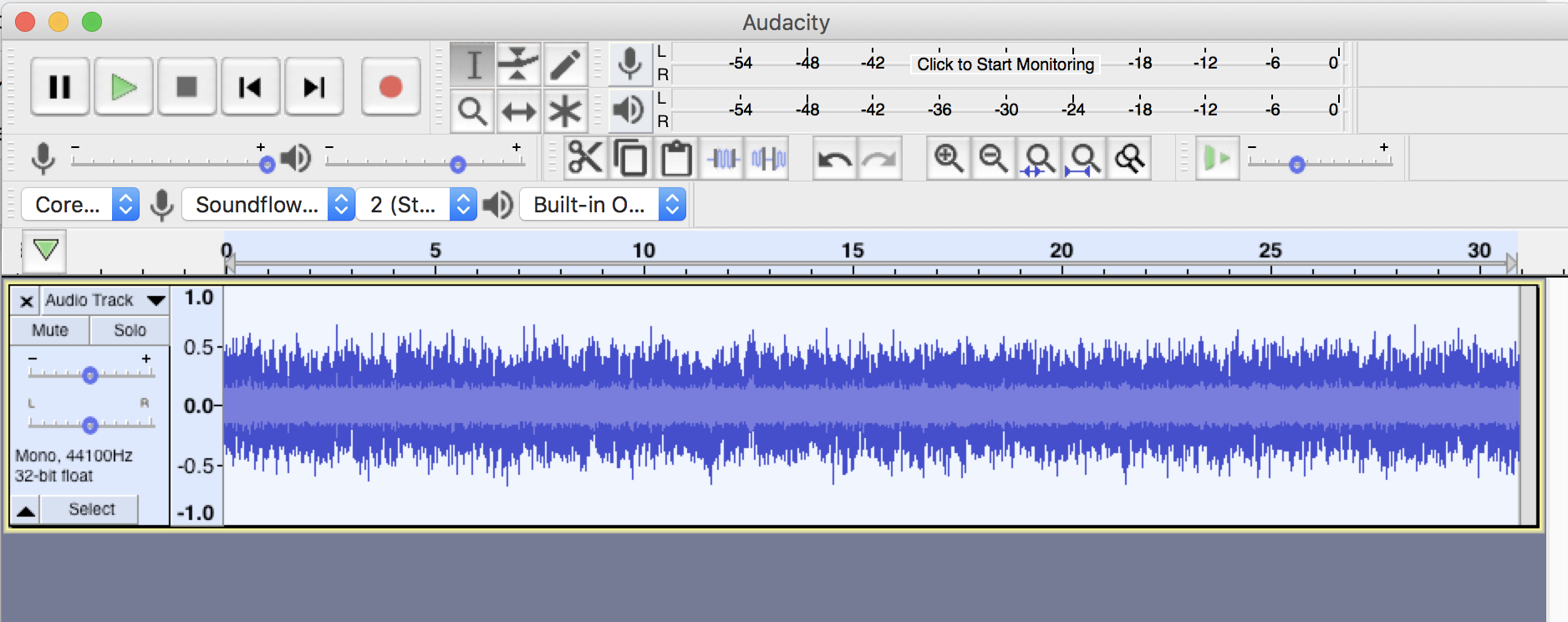
Figure 3. Track after generating pink noise.
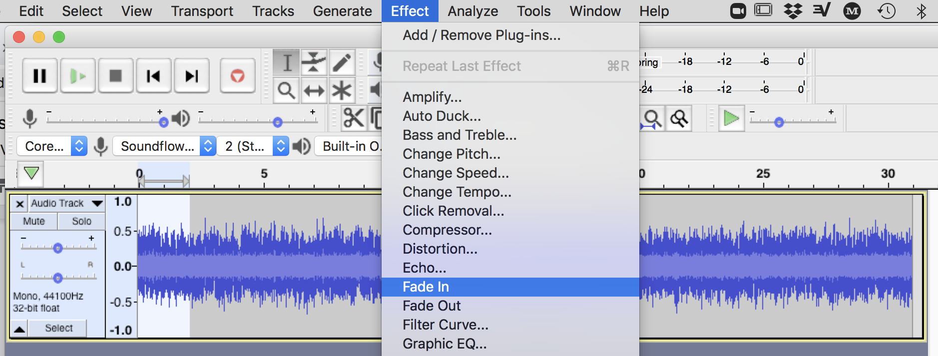
Next, we’ll need to add in fade-ins and outs. Without adding fades, at least one fade at the end, some digital distribution services (and ultimately some streaming service providers) will not accept the track as they do not allow hard ends to tracks. (note: if you are specifically creating a loopable track, then you should add “Loopable (No Fade)” to the track title to help get around this hard-cut moderation flag).
Figure 4. Add two-second fade-in in Audacity using Effect menu
Figure 5. Add two-second fade-out in Audacity using Effect menu
Export the track as .wav files 16-bit, 44.1k file. You may consider the export of the audio file as our “mixdown.” (Note: While some distribution services allow higher-quality tracks for import, our track settings get us close to our target output for this release). We are near finishing up our track, but we aren’t done. We should first listen to the audio file and then we may still want to “master” the track, or at the very least check out our loudness units (LUFS) relative to our target (streaming services) before preparing the file for distribution (footnote 2).
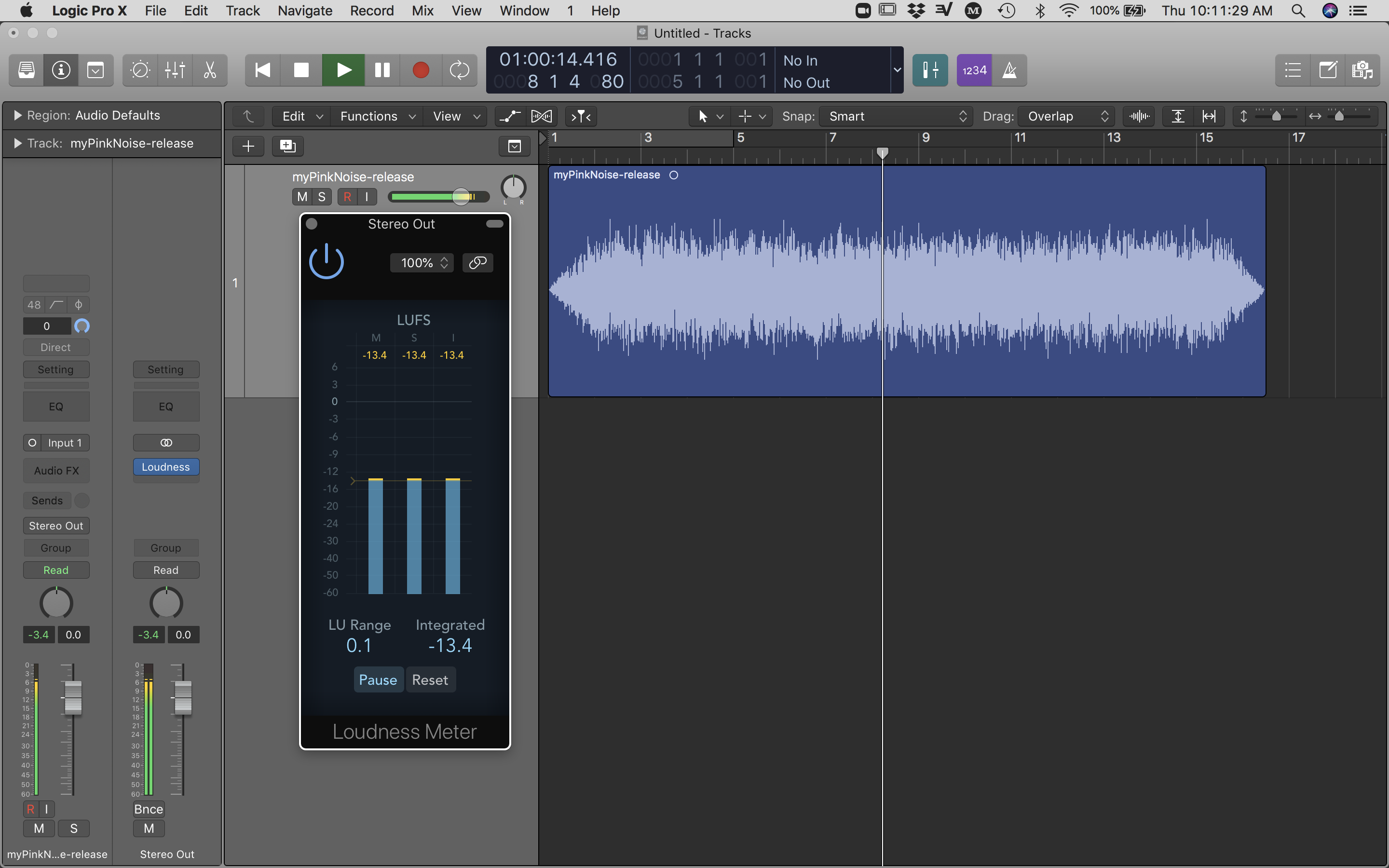
We can accomplish metering our track by opening our file inside any software that can meter LUFS and possibly control gain. If you need a free LUFS meter to quickly assess integrated LUFS, try Orban (url). Using Logic Pro X, I dragged and dropped the audio file onto the track and inserted a stock “Loudness Meter” plugin on the stereo buss. Playing back the track, the short-term and integrated meters are roughly -13.4dB LUFS. Since most streaming services use Integrated LUFS to alter the volume of tracks, a good range for most services is between -12 and -16dB LUFS. At the time of writing this, Spotify uses -14dB LUFS. (url) You may choose to alter the gain for the track or keep what you have. Since pink noise is already “mastered” in the production sense that it has equal energy per octave, I am choosing to not add any EQ, compression, or limiting, and I will instead stick with -13.4dB LUFS on my output meter.
Figure 6. Loudness Meter, measuring short-term and integrated LUFS.
If you did happen to alter the gain, you will either want to export out the “mastered” version as .wav or .aiff from your audio software or revisit Audacity to re-export another “mixdown” at a lower volume. Again, you will want to export out audio using uncompressed audio file formats (.wav or .aif), at least until you are ready to deliver to the distribution service.
2. GENERATE ALL MATERIALS ASSOCIATED WITH THE RELEASE
The materials for a release with a distributor include:
Audio file in the correct format (FLAC, .wav, .mp3, etc) and output target volume (e.g., -14dB LUFS)
Cover art for the single/EP/album
Track title
Artist name
Album/EP title (if necessary)
Choose a Genre (to categorize the music)
Label name (if any)
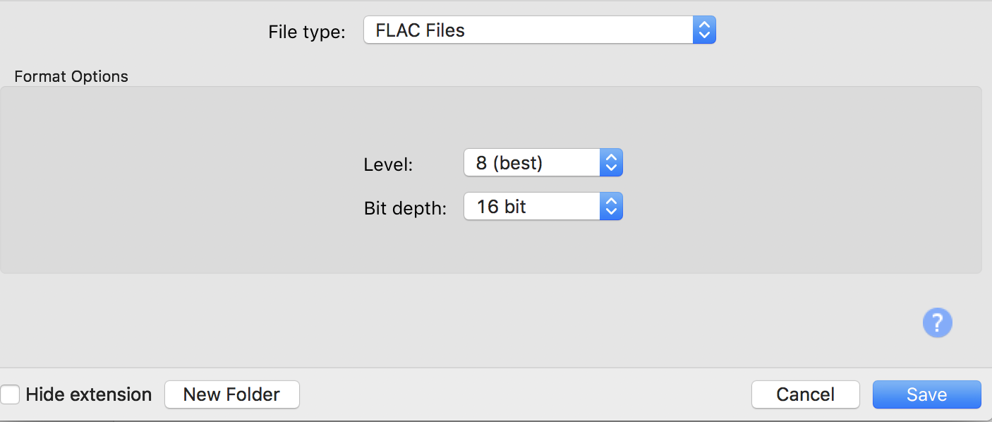
While we created a “mastered” version of the audio to be released, the target format may need to be altered before distribution. Services like CDBaby allow for uncompressed formats like .wav but others like RouteNote only take .flac or .mp3 file formats. Since FLAC is an uncompressed format and the distribution service for this walkthrough is RouteNote, let’s convert our “master” into a .flac file. Audacity software handles exporting out to this format. Just open up your mastered track in Audacity and export audio out as FLAC (footnote 3).
Figure 7. FLAC settings in the Export Audio window in Audacity software
Note: you do not want to convert to .mp3 for your release as this not only reduces the quality, but may introduce short bits of silence (10-20ms) at the beginning and end of your audio track(s). So for the case of “Loopable (No Fade)” tracks, .mp3 conversion can actually print silence into the track and cause a quick burst of amplitude rupture on streaming services due to the added silence from the codec compression conversion. This has nothing to do with buffering.
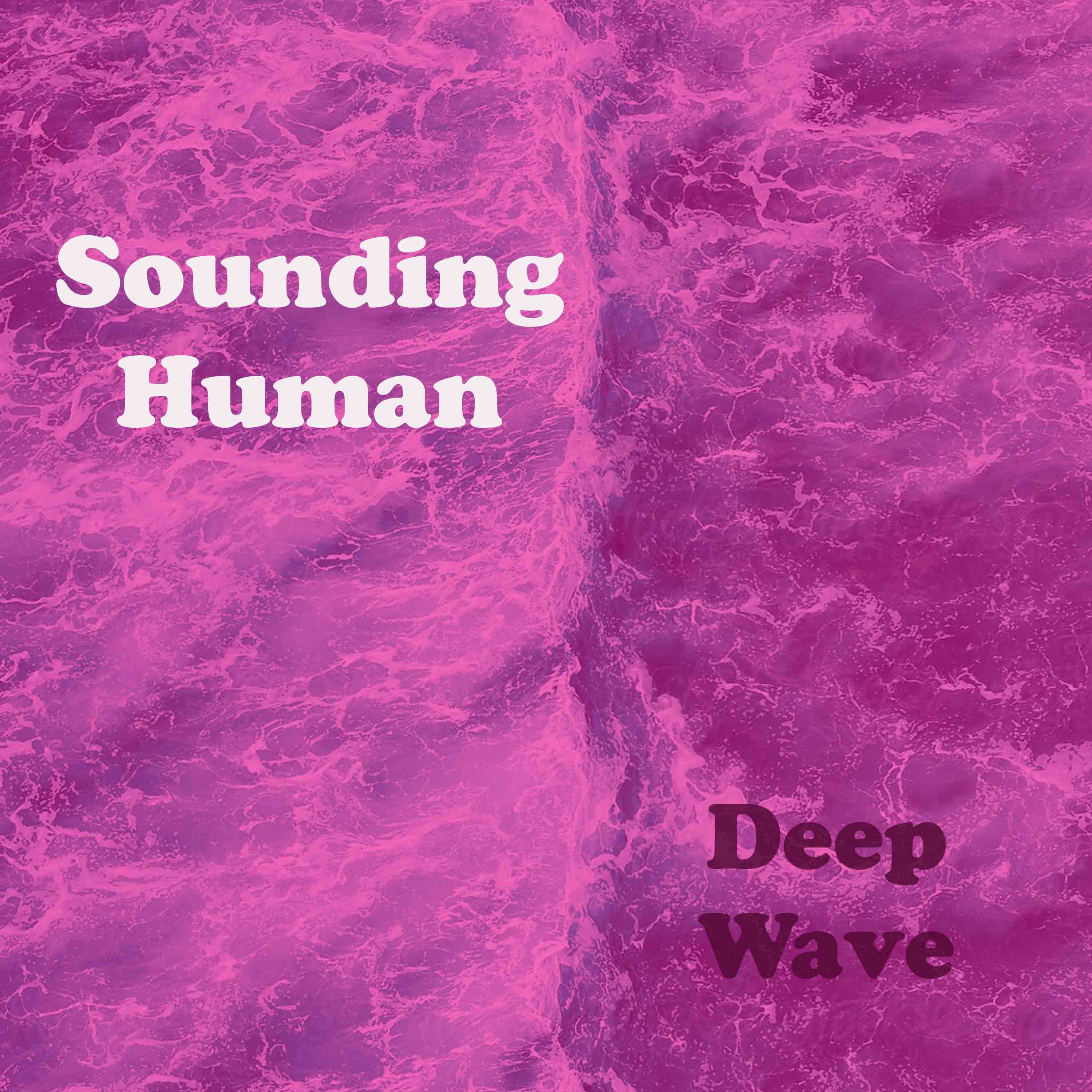
The cover art doesn’t need to be fancy, it just needs to fit the specifications. At the time of this writing, RouteNote has an image database that’s free to use and a photo resizer. If you want to make your own, RouteNote requires 3000×3000 pixel .jpg files. Just find your favorite pink color (RGB or Hex color) and fill a 3000×3000 pixel canvas with this color. I use Adobe Photoshop, but any free image editing software will do. Most other distributors also have free tools you may use to generate cover art. And should you choose to add images as part of your cover art, make sure you have permission first (again RouteNote has a free image database).
Figure 8. Color cover art (what I didn’t use but this image is 3000×3000 pixels!)
Figure 9. My 8-minute cover art for the release made in Photoshop
For this walkthrough, naming may be the hardest part. Maybe? Did I prime you to overthink it? Come up with an artist name and a track title. Just relax and let the word association flow. Seriously. Track titles can be anything— scientific “Equal Amplitude Per Octave”; direct “Pink Noise with fades”; spiritual “Soothing Pink Noise”; or cheeky, “Pink Panther’s Pink Noise”. The point is to pick a title and move on. The walk-through is about getting comfortable with the process, not to get bogged down by the details— that is, a “perfect” name. Sidenote: you cannot use “Untitled” or “No name” as these generic titles can be flagged by the distributor. You should do a quick word association for the artist name as well… remember, you never have to use your artist name again, but you must pick a name.
Afterward, you should get on a streaming service (here) (here) or (here) and do a quick check to make sure your new artist’s name doesn’t match existing artists (unique names make searching easier, and your work/streams will be attributed to you without added hassle).
Here’s what I came up with for my track (ie. You shouldn’t use. Now on Spotify)
Artist: Sounding Human Album/EP title: “Deep Wave” EP (can also be same name as your track) Track 1: “Deep Wave Pink Noise” and Track 2: “Deep Wave Pink Noise (Loopable, No Fade)”
Ready to move on? What? No?! Seriously? You don’t have a name yet? Use the letters from your name in this anagram maker. (url) Take one of the top five that appears. This is your artist name.
3. REGISTER WITH ROUTENOTE DISTRIBUTION SERVICE
Register with RouteNote. (url) On the RouteNote page, click on the “Join RouteNote” button. All you need is your email and a username. If you have an account already, just log in (footnote 4).
For any release, you have to pick a distribution service (DistoKid, RouteNote, CDBaby, Mondotunes, ReverbNation, Landr, Awal, Fresh Tunes, Tunecore, Chorus Music, Symphonic, etc). You don’t have to choose the same service in each release, but you cannot release the same music on multiple digital distribution providers. I’ve chosen RouteNote as it’s free to release, will keep your music up after you release, and satisfies the purposes of this walkthrough. Fun fact: you also can share revenue with this service. Please note that all distribution services take some sort of cut, whether upfront in fees, or later on in streaming. You always retain the rights to your music. For a full list comparing all the services check out Ari’s Take (url).
4. DISTRIBUTE YOUR WORK
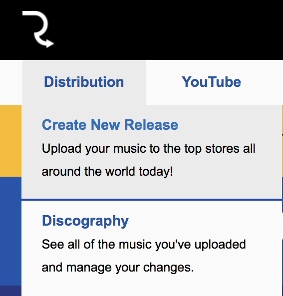
Ok. You’re ready to create your release with the distributor. Just log in to RouteNote and click Distribution > Create Release.
Figure 10. RouteNote Distribution menu
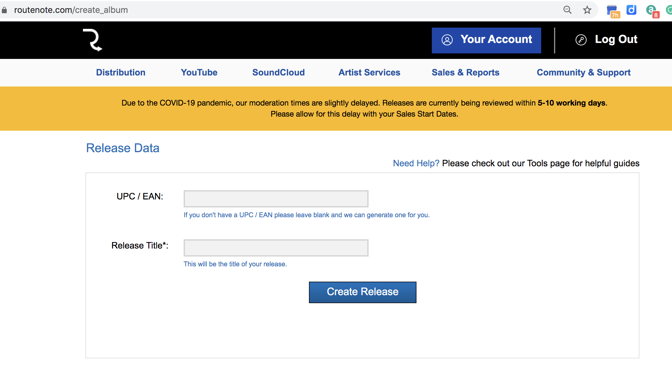
You’ll need to add your track title (or EP or Album title) to the release. Don’t worry about the UPC as RouteNote assigns you one for free. A UPC is a universal product code associated with the release. Think of it like a barcode that you see on a CD or LP. The UPC is specific to YOUR single/EP/album. Some services, like CDBaby, charge for this. It’s free here.
Figure 11. RouteNote initial Release Data input fields
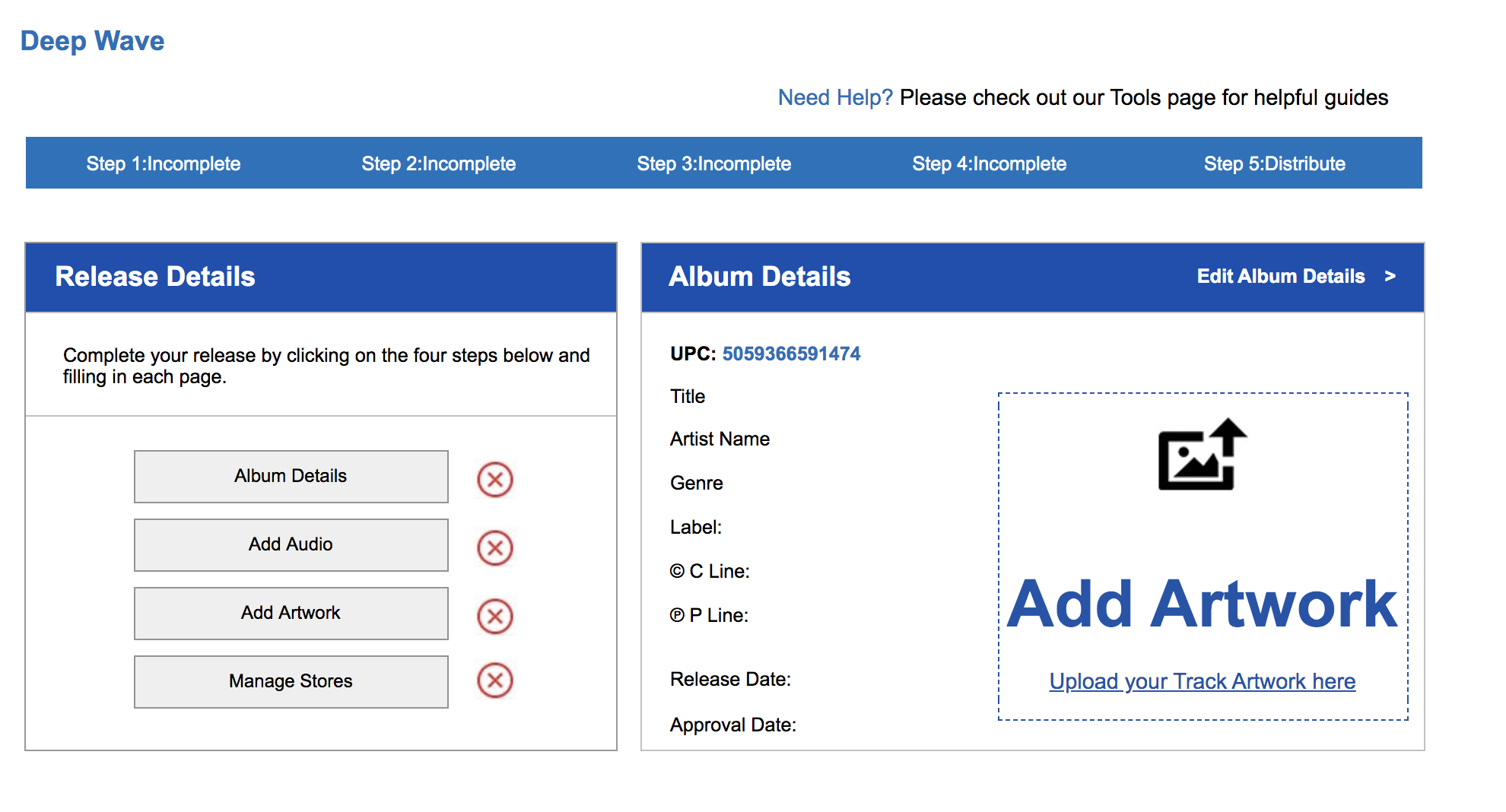
After the initial title name and receiving a UPC, there’s a four-step process to the release that we have prepped for in step 2.
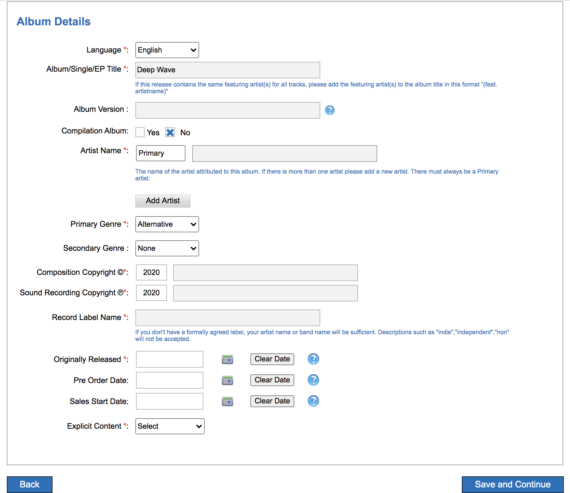
1. Album Details. See the image below for all fields. You may choose to use your own name for C and P copyright, although you may use the artist name. C is for the underlying composition (the written music) and P is for the recording (what the artist records). Often, the C and P lines on the record are attributed to the record label (e.g., Sub Pop, Matador), but not always. You’ll also need a genre, but for something like pink noise, maybe “Easy Listening”? A note about release date. If you are setting this up for music release, you’ll want to time this in advance and have an album release strategy. As Bobby Schenk, digital marketing manager for Dub-Stuy records, puts it, “Include the 7-10 day delay in your release strategy. Release earlier rather than later with a scheduled release, as you’ll need to align with your PR machine.”
Figure 13. RouteNote Album details screen
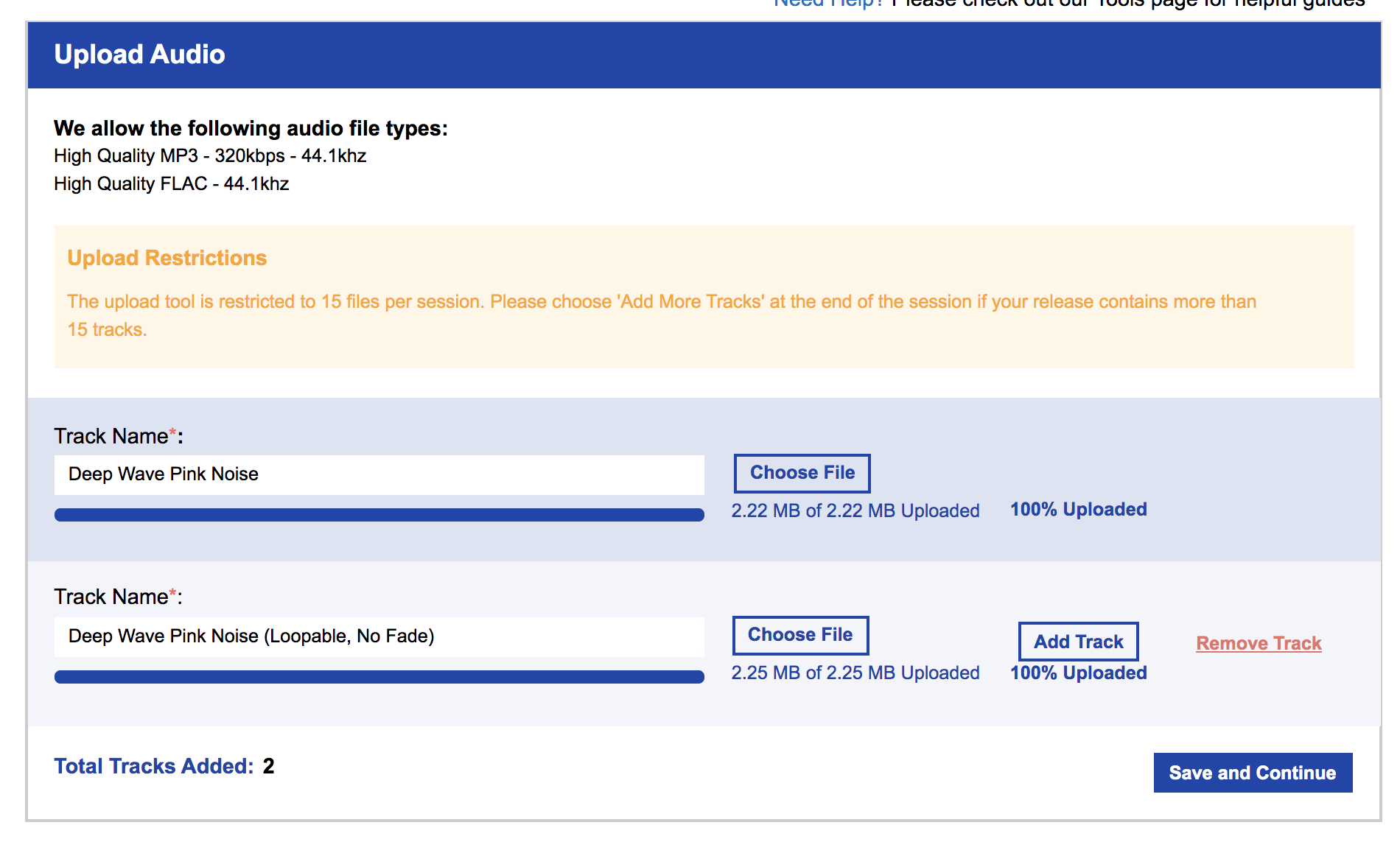
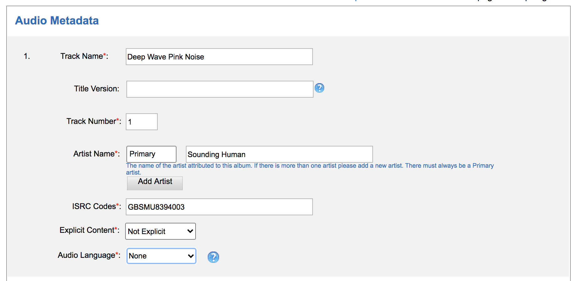
2. Add Audio. This is where you’ll upload ALL audio files. You’ll need the track name, but you’ll be asked to assign some additional metadata to each track (if you’re uploading more than one track). Since the track is pink noise with no lyrics, there will be no language associated with the track. Your track will be assigned an ISRC (‘International Standard Recording Code’) and that ISRC is attached to the recording, not the underlying composition. ISRCs are one important way for tracking streams (read royalties) as they are individual barcodes to the musical recordings. Read about ISRC (url). Read more on composition vs recording (url).
Figure 14. RouteNote Upload Track screen
Figure 15. RouteNote Track Metadata screen
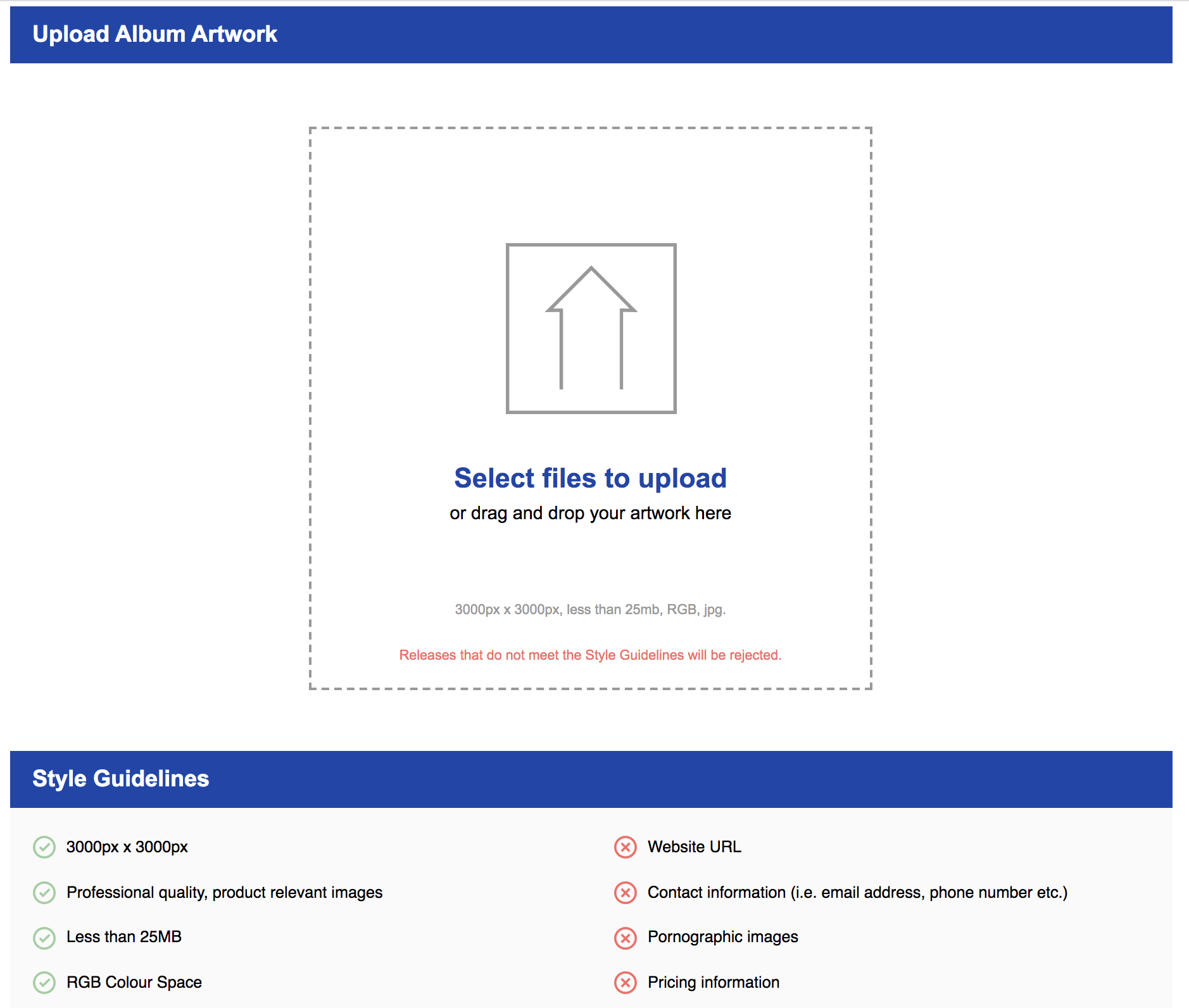
3. Add Artwork. We’re halfway there! Next, we need to upload our album/single cover art. Remember, the guidelines are hi-resolution files, and for RouteNote that is 3000×3000 jpg files only.
Figure 16. Route Upload artwork Screen
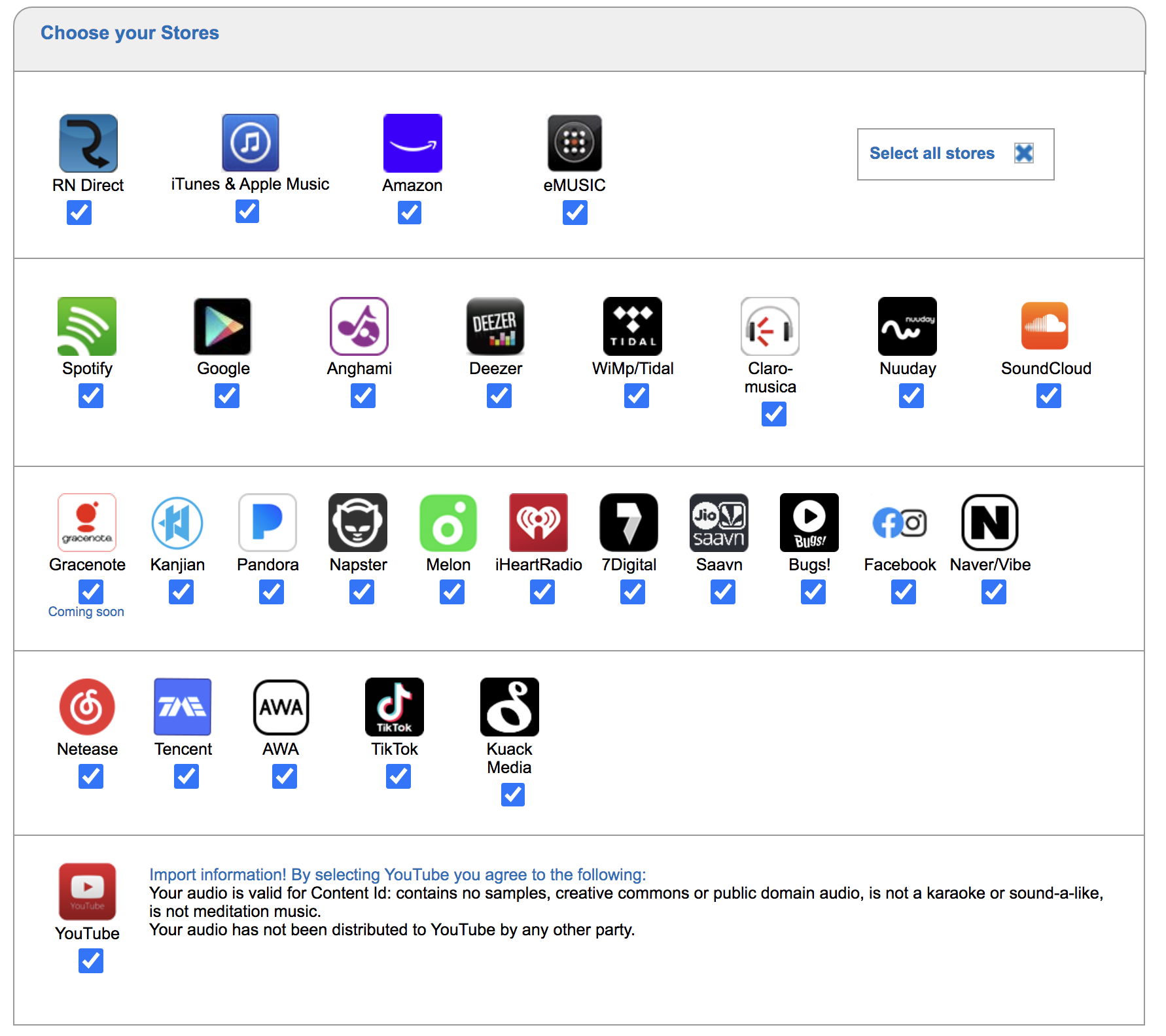
4. Choose Your Stores. This part should be simple. What services do you want your music on? Spotify? YouTube? Tidal? All? You can be picky but often the default is to distribute on all platforms all over the world. RouteNote makes it easy with one button-click.
Figure 17. RouteNote Store selection screen
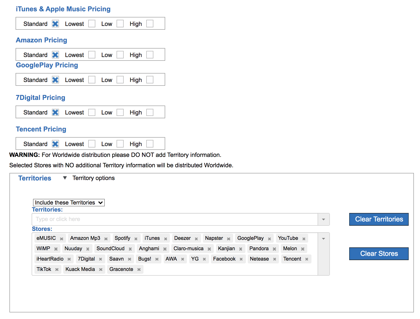
Figure 18. RouteNote Territories selection screen
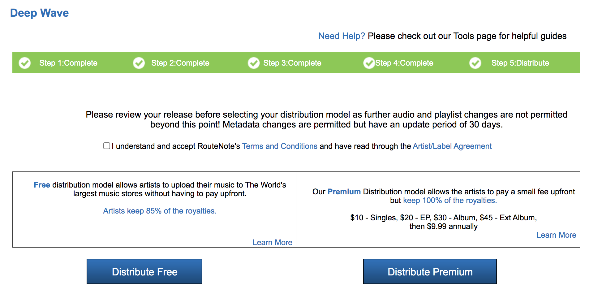
Now you’re ready to distribute! All you need to do is check over your work and then click on “Distribute Free.” And that’s it! RouteNote will take a cut of your streams (15%) but there are no upfront costs to the process.
Figure 19. RouteNote Completion Screen. Two options for distribution (free vs paid).
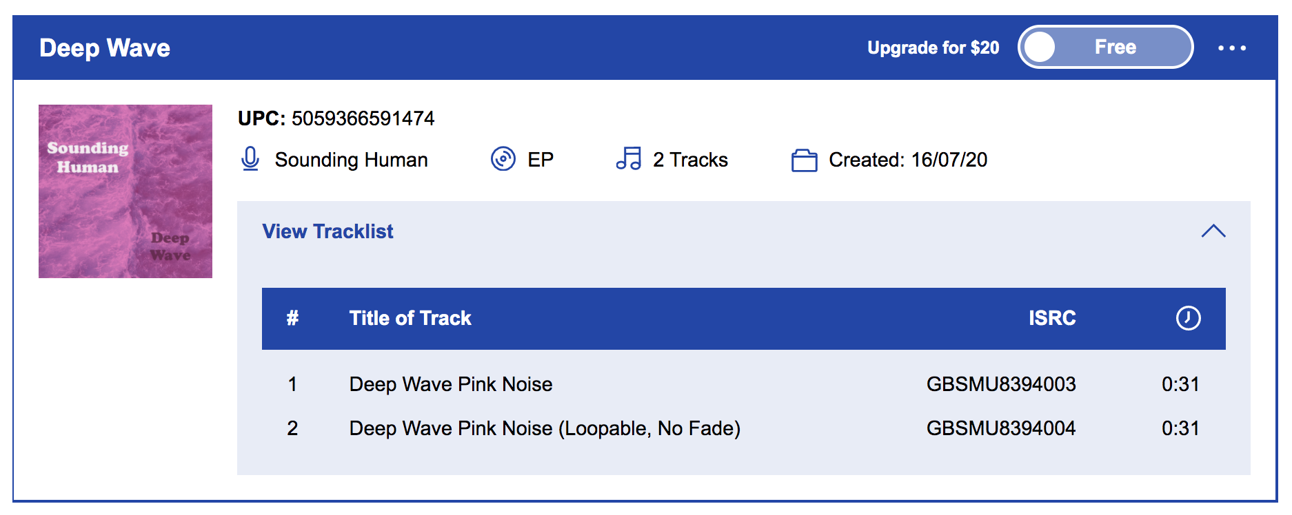
Figure 20. RouteNote Post-Distribution. In Review details
5. NOW WHAT?
The release will take about a week or so to be released, at which point you should receive an email. If there are issues with your work (track titles too generic, audio file has copyright issues, etc.) you will receive an email in which you’ll need to resolve all issues before the release can move forward (footnote 5).
While you wait for your release to go through moderation, here are a few things you’ll want to consider as part of any release that you do in the future. Maybe not part of this walkthrough, but certainly if you are getting serious about releasing your music.
1. Check out new music. Listen to the walkthrough release, Sounding Human, on Spotify, 🙂
2. Register your work(s) with a Performing Rights Organization (PRO)
If you’re not already part of a PRO (ie., ASCAP, BMI) you should strongly consider it. …. You’ll need to be registered with a PRO in order to register your work for admin publishing royalties among other things. Here’s some reading about PROs (url) (url). Quick note: A composition can have multiple recordings (ISRCs), but only one composition (ISWC). What’s an ISWC? Read here (URL).
3. Register your work on SoundExchange
At this point, your music will appear on streaming platforms that have two types of plays (interactive and non-interactive). Interactive streams are where people hit the play button on your music (or if it’s on a playlist. However, digital distribution services like RouteNote cannot collect on non-interactive streams (radio-type play). SoundExchange (url) is the collector of these royalties. Registration is free, but you’ll need to upload and claim all your recordings if you want to collect within this market. Want to learn more about this? Read here (URL)
4. Claim your Artist Profile
After your release is live, you’ll want to decide if you want to claim your artist profile. Doing so allows you to update profile pic, add a bio, create artist playlists, and even track who is listening to your music every day. Claim your artist on Apple (url), Spotify (url), Amazon (URL).
5. Start a Digital Store
Some services offer you to sell your music directly to fans/consumers, but many are not digital stores. In this case, you may consider a digital store like Bandcamp (url), where you can sell your music as direct downloads, all from one location.
That’s basically it! In one hour or one pot of coffee (hopefully that’s all it took), you’ve gone from zero to release. If you dug this walkthrough, please share, follow my music on Spotify (url), and pay it forward in your own musical community. Thanks for being an active participant!
Footnotes:
1. 30 seconds for a stream count seems to be an agreed-upon time length. I ran a test on my EP Software 1.17 (Spotify link) with the final track clocking in at 26 seconds. After a year and with friends streaming this track across multiple services, the track still has 0 plays for royalties. If you want to dig deeper on Spotify’s algorithm, which helps support the 30-second rule, check out this article (url).
2. Streaming services typically average -12dB to -16dB Integrated LUFS (loudness units to full scale). All streaming services use LUFS to act as your own personal DJ, helping adjust the volume between tracks that may be coming from a different genre, era, or artist. It’s become more common that Spotify uses -14dB LUFS for its target. This means you that if you crush your track with an integrated LUFS (overall average loudness) of -8dB, Spotify can very well turn your track down by -6dB making it half as loud… meaning you lose all that intensity you spent so hard to work for. Use a meter! (url)
3. Make sure you always listen to your work after you export it! You want to make sure everything sounds correct before you upload your audio file. Do NOT distribute without listening to your final work first.
4. RouteNote registration full disclosure. I included a referral link for registering with RouteNote in step 3. Referral ID: 2f79120f. You get your full cut regardless; RouteNote simply takes a percentage of their own earnings and passes it on to me. Thank you for supporting articles like this with using the referral code.
5. Note for our walkthrough that releasing a noise track via RouteNote will not appear on Apple Music / iTunes. I inquired with RouteNote directly, and here’s what their moderation team had to say (email dated 7/24/2020), “Unfortunately iTunes no longer accept white noise/nature sounds content due to the high amount that was being uploaded to them. They have asked us to no longer send it to them, for this reason the store was blocked.” If you go through a different distribution service, you can get noise albums on Apple Music (case in point, here’s an album I created for an Oregon-based birth center: https://music.apple.com/us/album/calming-sounds-for-pregnancy-birth-and-parenting/1522834278)